Machine Learning · Insper · E2.2

TF-IDF

Fundamental approach

Term frequency × inverse document frequency: by hand, in scikit-learn and in a search engine

Where the bag-of-words left us

words that are everywhere

"the"

in 9,475 of the 11,314 posts

one strange document

"ax"

62,387 occurrences, in 20 posts

A stop list fixes the first problem, for one language and only for the words someone thought of listing.

Predict. What single rule, learned from the corpus itself, could fix both problems?

The path of this part

Weigh the wordstf × idf, the idf curve
Compute and checkthree sentences by hand, then scikit-learn
Compare and searchcosine, a small search engine, a real corpus

Each stage answers one question: how much should a word weigh? → where does each number come from? → which texts are alike, and which answer a query?

Stage 1 · how much should a word weigh?

The idea

Spärck Jones (1972): a term that occurs in many documents is a poor way to tell documents apart, so it should count less.

A word weighs more in a document the more often it occurs there, and less the more documents contain it.

Salton & Buckley (1988), comparing many weighting schemes, made tf × idf with length normalization the standard of information retrieval.

scikit-learn's version

\[ \text{tf-idf}(t, d) = \underbrace{\text{tf}(t, d)}_{\text{count of } t \text{ in } d} \times \underbrace{\Big(\ln \frac{1 + n}{1 + \text{df}(t)} + 1\Big)}_{\text{idf}(t)} \]

\(n\) documents, \(\text{df}(t)\) of them contain \(t\). Then every row is divided by its length (norm='l2').

"+1" inside the fraction

smooth_idf=True: as if one extra document contained every word once. No division by zero.

"+1" outside

a word in every document keeps weight 1, not 0: discounted, not deleted.

The idf curve

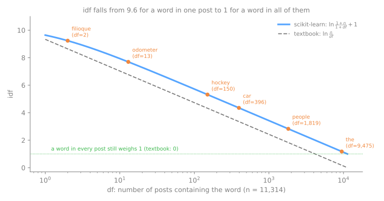
idf against the number of posts containing the word, for n = 11,314 posts: scikit-learn's curve falls from 9.6 for a word in one post to 1 for a word in all of them, while the textbook ln(n/df) reaches 0

"filioque", in 2 posts: idf 9.2

"the", in nearly all: idf 1.18

Logarithmic: going from 1 post to 10 costs about as much weight as going from 1,000 to 10,000.

Stage 2 · where does each number come from?

TF-IDF by hand, step by step

The counts of the bag-of-words page, \(n = 3\) documents: df, the idf values, then each row (tf × idf, its length, the division). Predict. How many different idf values can there be? Which word of d1 will weigh most?

Counts against TF-IDF

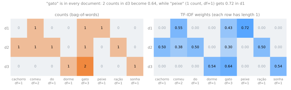
Two heatmaps of the same three documents. Counts: gato has 2 in d3. TF-IDF: gato, present in every document, drops to 0.43 in d1 and 0.30 in d2, while peixe, in one document, gets 0.72

In d1 and d2, "gato" now has the smallest non-zero weight: it is everywhere.
In d3 it still has the largest (0.64): it occurs twice, and tf still counts.

The weighting does not remove common words; it lowers them relative to rare ones.

Stage 3 · which texts are alike, and which answer a query?

Comparing documents: the cosine is a dot product

TF-IDF rows have length 1, so the cosine is just their dot product. d1 and d2 share comeu and gato:

\[ \cos(d_1, d_2) = 0.5478 \times 0.3838 + 0.4254 \times 0.2980 = 0.2102 + 0.1268 = 0.337 \]

d1 and d3 share only gato: \(0.4254 \times 0.6411 = 0.273\).

Predict. With raw counts the same pairs had 0.516 and 0.471. Did every similarity go down? Which pair dropped the most?

Every similarity went down

counts


       d1     d2     d3
d1  1.000  0.516  0.471
d2  0.516  1.000  0.365
d3  0.471  0.365  1.000

TF-IDF


       d1     d2     d3
d1  1.000  0.337  0.273
d2  0.337  1.000  0.191
d3  0.273  0.191  1.000

Every shared word here includes "gato", which TF-IDF discounts. d1–d3 dropped the most (0.471 → 0.273): what they share is only "gato", the least informative word.

A small search engine

A help-desk FAQ of ten questions. Turn the query into a vector with the same fitted vectorizer, rank the questions by cosine.

"esqueci minha senha" (I forgot my password)
"erro 0x80004005" (an error code)
"quero contestar a correção do exame" (I want to contest the grading of the exam)
"onde almoçar no sábado" (where to have lunch on Saturday)
"perdi a fatura" (I lost the invoice)

Predict. Which of the five will find the right question?

Two work, three fail

query	score	best match	words used
esqueci minha senha	0.35	FAQ 0: trocar a senha…	senha
erro 0x80004005	0.53	FAQ 9: o erro 0x80004005…	erro, 0x80004005
quero contestar a correção do exame	0.51	FAQ 0: trocar a senha…	do
onde almoçar no sábado	0.37	FAQ 2: segunda via do boleto…	onde
perdi a fatura	0.00	FAQ 0 (first by default)	—

A rare token has a high idf: an exact code is the ideal TF-IDF query.
"contestar a correção do exame" shares only "do"; the right answer ("revisão da nota de uma prova") uses none of its words.
The restaurant entry says "sábados", not "sábado": a stemmer would fix that one.

A stop list removes false matches, but cannot create true ones


quero contestar a correção do exame   best score 0.00
onde almoçar no sábado                best score 0.00

With the function words gone, TF-IDF honestly says it found nothing. Keyword search can only be as good as the overlap between the words of the query and the words of the documents.

On a real corpus

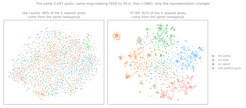
t-SNE maps of the same 2,097 posts from four newsgroups. With raw counts the colors are mixed and 46% of each post's 5 nearest neighbors come from its own newsgroup; with TF-IDF four colored regions appear and the figure is 81%

2,097 posts from four newsgroups, reduced with a truncated SVD (singular value decomposition) and drawn with t-SNE (t-distributed stochastic neighbor embedding; the color is the newsgroup). Nearest 5 posts from the same newsgroup: counts 46%, TF-IDF 81% (random: about 25%).

Simulator: TF-IDF and search, live

Predict. In the lesson preset, untick smooth_idf: will the idf of the rare words go up or down? Then try the synonyms preset.

Summary

idf discounts words by the number of documents that contain them; tf still counts repetitions.
scikit-learn: \(\ln\frac{1+n}{1+\text{df}} + 1\), then each row divided by its length.
Rows of length 1: the cosine is a dot product.
Search: the same fitted vectorizer for documents and query; exact rare tokens are its strength.

Fundamental lab · about 25 min, in pairs

The TF-IDF matrix of real posts, steps 1 to 5

The same four newsgroups as the bag-of-words lab, about 2,100 posts; scikit-learn only.
Steps: load the posts · the matrix and its idf · what a post is about, in eight words · the most similar posts · which options give the best neighbors.
At every step, answer the Predict before running. Simulation: counts against TF-IDF, for one post (step 3).
Download the lab notebook and open it in Jupyter or Colab.

Pace: steps 1 and 2 in 5 min; step 3 and the simulation in 8 min; steps 4 and 5 in 12 min.