U4.3 Word Embeddings

Bag-of-words and TF-IDF give every word its own column. The columns are orthogonal, so "car" and "automobile" are exactly as unrelated as "car" and "banana": the representation knows which words a document contains, and nothing about what those words mean. A word embedding replaces the column with a short, dense vector (50 to 300 numbers) learned from a large amount of text, arranged so that words used in similar ways get similar vectors.

This page builds word vectors three ways, from the simplest to the most used. First by hand: count which words appear next to which on eleven sentences, reweight the counts, and compress them with the same truncated SVD you used in dimensionality reduction. Then word2vec, which learns the vectors by prediction, and its cousins GloVe and fastText. Then pretrained vectors, trained by someone else on billions of words, which you download and explore: nearest neighbors, similarities, the famous analogies (measured honestly, with the misses), the social biases they absorb, and the limit that motivates the next page: one vector per word, whatever the sense. Every number below comes from running the code next to it; the overview places this page among the four approaches.

The lesson follows one pipeline in four stages, drawn below: 1. context → meaning, the idea that a word is known by its neighbors; 2. count and compress, from co-occurrence counts to dense vectors; 3. learn by predicting, with word2vec and its cousins; 4. explore the space, with pretrained vectors, their analogies, their biases and their limit. Each stage links to its section, and in the slides a strip at the bottom shows which stage you are in.

Slides

Click the slides and use the ← → arrows to navigate; F goes full screen and Esc shows every slide. Open the slides in a new tab

The distributional hypothesis

Stage 1. Read these four sentences about a word you have never seen:

• Um copo de tiquira gelada. (A glass of cold tiquira.)
• A tiquira é feita de mandioca fermentada. (Tiquira is made from fermented cassava.)
• Bebeu tiquira demais e passou mal. (He drank too much tiquira and felt sick.)
• No Maranhão, servem tiquira nas festas. (In Maranhão they serve tiquira at parties.)

You now know that tiquira is an alcoholic drink, probably strong, from the north-east of Brazil, although nobody defined it. You inferred it from the company it keeps: glass, cold, fermented, drank, too much, parties. Words that appear in those contexts are drinks. This is the distributional hypothesis: words that occur in similar contexts tend to have similar meanings (Harris, 1954), or in Firth's (1957) phrase, "you shall know a word by the company it keeps".

The hypothesis turns meaning into something you can count. If two words keep appearing next to the same neighbors, their vectors should be close. Everything on this page is a way of turning "which words appear next to which" into vectors.

From co-occurrence counts to vectors

A toy corpus and its co-occurrence matrix

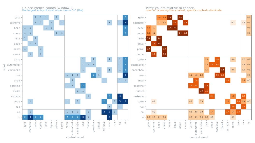
Stage 2. Eleven short Portuguese sentences: animals that eat and drink, and vehicles that run on fuel. The corpus is designed so that some pairs of words (gato/cachorro, carro/automóvel) never appear in the same sentence but share their neighbors. For each word, count how often every other word appears within a window of two words to its left or right:

import numpy as np
import pandas as pd

corpus = ["o gato bebe leite", "o gato come peixe",                  # the cat drinks milk / eats fish
          "o cachorro bebe água", "o cachorro come carne",           # the dog drinks water / eats meat
          "o cachorro corre na rua",                                 # the dog runs in the street
          "o carro usa gasolina", "o carro corre na estrada",        # the car uses petrol / runs on the road
          "o automóvel usa gasolina", "o automóvel anda na estrada",  # the automobile ... / goes on the road
          "o caminhão usa diesel", "o caminhão corre na estrada"]     # the truck uses diesel / ...
sentences = [s.split() for s in corpus]
vocab = sorted({w for s in sentences for w in s})
idx = {w: i for i, w in enumerate(vocab)}

window = 2
C = np.zeros((len(vocab), len(vocab)), dtype=int)     # rows: words · columns: context words
for s in sentences:
    for i, w in enumerate(s):
        for j in range(max(0, i - window), min(len(s), i + window + 1)):
            if j != i:
                C[idx[w], idx[s[j]]] += 1

print(len(vocab), 'words ·', C.sum(), '(word, context) pairs')
for w in ['gato', 'cachorro', 'carro', 'automóvel']:
    print(f"{w:10s}", {vocab[j]: int(C[idx[w], j]) for j in np.flatnonzero(C[idx[w]])})

20 words · 126 (word, context) pairs
gato       {'bebe': 1, 'come': 1, 'leite': 1, 'o': 2, 'peixe': 1}
cachorro   {'bebe': 1, 'carne': 1, 'come': 1, 'corre': 1, 'na': 1, 'o': 3, 'água': 1}
carro      {'corre': 1, 'gasolina': 1, 'na': 1, 'o': 2, 'usa': 1}
automóvel  {'anda': 1, 'gasolina': 1, 'na': 1, 'o': 2, 'usa': 1}

Check one row by hand. "gato" appears in two sentences. In "o gato bebe leite", the window of two words around it holds o, bebe and leite; in "o gato come peixe" it holds o, come and peixe. So o is counted twice and the others once: exactly the row printed. The matrix is 20 × 20: one row per word, one column per possible context word, and each row is that word's context profile.

Documents versus contexts: the bridge from bag-of-words

The bag-of-words matrix also has one column per word, but its rows are documents. Compare the two ways of describing a word, its column in the bag-of-words (which sentences contain it) and its row in the co-occurrence matrix (which words surround it), with the cosine similarity from the TF-IDF page:

from sklearn.feature_extraction.text import CountVectorizer

def cos(u, v):
    return u @ v / (np.linalg.norm(u) * np.linalg.norm(v))

D = CountVectorizer(token_pattern=r'\S+', vocabulary=vocab).fit_transform(corpus).toarray()
print('bag-of-words matrix:', D.shape, '(sentences x words)')
pairs = [('gato', 'cachorro'), ('carro', 'automóvel'), ('gato', 'carro')]
for a, b in pairs:
    print(f"{a:5s} / {b:9s}   bag-of-words columns {cos(D[:, idx[a]], D[:, idx[b]]):.2f}   "
          f"co-occurrence rows {cos(C[idx[a]], C[idx[b]]):.2f}")

bag-of-words matrix: (11, 20) (sentences x words)
gato  / cachorro    bag-of-words columns 0.00   co-occurrence rows 0.73
carro / automóvel   bag-of-words columns 0.00   co-occurrence rows 0.87
gato  / carro       bag-of-words columns 0.00   co-occurrence rows 0.50

As bag-of-words columns, all three pairs score 0.00: no sentence contains both words. As context rows, "carro" and "automóvel" score 0.87, because both are followed by usa gasolina and na. This is the whole idea in one table: similar words rarely appear together, but they appear next to the same words.

The last row shows the problem that remains. "gato" and "carro" score 0.50, only a little below the cat and the dog (0.73). Every noun of the corpus comes right after the article o, so every noun row has a large count in the o column, and that shared, uninformative count dominates the cosine. The same thing happens on real text with the, of and de.

PPMI: counting what is surprising

The fix is to ask not "how often do w and c appear together?" but "how much more often than chance?". If the word and the context were independent, the pair would appear with probability \(P(w)\,P(c)\). The pointwise mutual information compares the observed probability with that (Church & Hanks, 1990):

where \(n(w, c)\) is the count in the cell, \(n(w)\) the row total, \(n(c)\) the column total and \(N\) the total of the matrix. PMI is 0 when the pair appears exactly as often as chance predicts, positive when more often. By hand, for two cells of the "gato" row:

N = C.sum()
n_word = C.sum(axis=1)          # how often each word is a center word
n_ctx = C.sum(axis=0)           # how often each word is a context
for w, c in [('gato', 'bebe'), ('gato', 'o')]:
    n = C[idx[w], idx[c]]
    pmi = np.log2(n * N / (n_word[idx[w]] * n_ctx[idx[c]]))
    print(f"PMI({w}, {c}) = log2({n} x {N} / ({n_word[idx[w]]} x {n_ctx[idx[c]]})) = {pmi:.2f}")

PMI(gato, bebe) = log2(1 x 126 / (6 x 6)) = 1.81
PMI(gato, o) = log2(2 x 126 / (6 x 22)) = 0.93

In raw counts, o was the strongest context of "gato" (2 against 1). In PMI the order flips: o appears 22 times as a context, next to everything, so seeing it next to "gato" is barely surprising (0.93), while bebe appears only 6 times and 1 of them is with "gato" (1.81). Pairs never seen have \(\log 0 = -\infty\), and negative PMI values are unreliable with small counts, so the standard choice is to clip them to zero: positive PMI, \(\text{PPMI} = \max(\text{PMI}, 0)\).

with np.errstate(divide='ignore'):                 # log2(0) = -inf for pairs never seen
    PMI = np.log2(C * N / np.outer(n_word, n_ctx))
PPMI = np.maximum(PMI, 0)
for w in ['gato', 'cachorro']:
    print(f"{w:9s}", {vocab[j]: round(float(PPMI[idx[w], j]), 2) for j in np.flatnonzero(PPMI[idx[w]])})
for a, b in pairs:
    print(f"{a:5s} / {b:9s}   counts {cos(C[idx[a]], C[idx[b]]):.2f}   PPMI {cos(PPMI[idx[a]], PPMI[idx[b]]):.2f}")

gato      {'bebe': 1.81, 'come': 1.81, 'leite': 3.39, 'o': 0.93, 'peixe': 3.39}
cachorro  {'bebe': 1.22, 'carne': 2.81, 'come': 1.22, 'corre': 0.22, 'na': 0.22, 'o': 0.93, 'água': 2.81}
gato  / cachorro    counts 0.73   PPMI 0.22
carro / automóvel   counts 0.87   PPMI 0.75
gato  / carro       counts 0.50   PPMI 0.05

The o column is now one of the smallest in each row, and "gato"/"carro" falls from 0.50 to 0.05: the similarity that came from the article is gone. But so is much of the similarity between the cat and the dog, which drops from 0.73 to 0.22. The two animals share only bebe and come; their other contexts (leite, peixe, água, carne) are four different words, and in a 20-column space four different words are four orthogonal directions. The PPMI rows are right about what is informative, but too literal: they do not know that milk, water, fish and meat are themselves similar.

(figure script)

Truncated SVD: from 20 sparse columns to 2 dense numbers

Compressing the PPMI matrix is what connects "milk" to "water": they get similar vectors because the words around them (bebe, and the animals) are the same. The tool is the truncated SVD, the version of PCA that works on a matrix without centering it. It keeps the \(k\) directions that explain most of the matrix and gives every word \(k\) coordinates. With \(k = 2\):

from sklearn.decomposition import TruncatedSVD

svd = TruncatedSVD(n_components=2, random_state=0)
Z = svd.fit_transform(PPMI)                        # one row of 2 numbers per word
print(pd.DataFrame(Z, index=vocab, columns=['dim 1', 'dim 2'])
        .loc[['gato', 'cachorro', 'leite', 'carro', 'automóvel', 'gasolina', 'o']].round(2))

table = pd.DataFrame({
    'BoW columns': [cos(D[:, idx[a]], D[:, idx[b]]) for a, b in pairs],
    'counts': [cos(C[idx[a]], C[idx[b]]) for a, b in pairs],
    'PPMI': [cos(PPMI[idx[a]], PPMI[idx[b]]) for a, b in pairs],
    'PPMI + SVD': [cos(Z[idx[a]], Z[idx[b]]) for a, b in pairs]},
    index=[f"{a} / {b}" for a, b in pairs])
print(table.to_string(float_format=lambda v: f"{v:.2f}"))

           dim 1  dim 2
gato        3.77  -0.97
cachorro    2.55  -0.35
leite       2.78  -0.79
carro       0.61   1.87
automóvel   0.70   2.28
gasolina    0.64   2.44
o           1.77   1.05
                   BoW columns  counts  PPMI  PPMI + SVD
gato / cachorro           0.00    0.73  0.22        0.99
carro / automóvel         0.00    0.87  0.75        1.00
gato / carro              0.00    0.50  0.05        0.06

Read the first table: every animal-and-food word has a large first coordinate and a negative second one, every vehicle-and-fuel word the opposite. The two numbers are a dense word vector. Nobody told the SVD which words are animals: it found the two directions because the two groups of words share contexts inside each group and not across.

The second table is the story of this section in four columns. The bag-of-words sees nothing (0.00 everywhere). The raw counts see everything as similar, including cat and car (0.50). PPMI removes the article but becomes too literal (cat/dog 0.22). PPMI followed by SVD gets all three pairs right: cat/dog 0.99, car/automobile 1.00, cat/car 0.06.

(figure script)

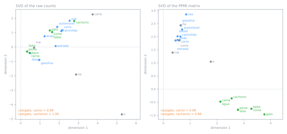
The left panel is the SVD of the raw counts: the first direction just measures frequency (the article o sits far out alone), and animals and vehicles are mixed along it. The right panel is the SVD of PPMI.

This recipe (count co-occurrences in a window, reweight with PPMI, reduce with SVD) is a complete method for word vectors, and it is still competitive: the lab applies it to one million words of Wikipedia in a few seconds and compares it with the methods below. On a real corpus the matrix has thousands of rows and \(k\) is 100 to 300; it is the same code with a sparse matrix.

The same compression on documents: latent semantic analysis

The first dense word vectors in wide use did not even need a window. Latent semantic analysis (LSA, Deerwester et al., 1990) applies the truncated SVD directly to the TF-IDF matrix of the TF-IDF page. Read column by column, that documents × words matrix describes each word by the documents it appears in, which is the "bag-of-words columns" view above; the SVD compresses those columns into short dense vectors. On the 11,314 training posts of 20 Newsgroups, the corpus of the other text pages, with 100 components:

(figure script)

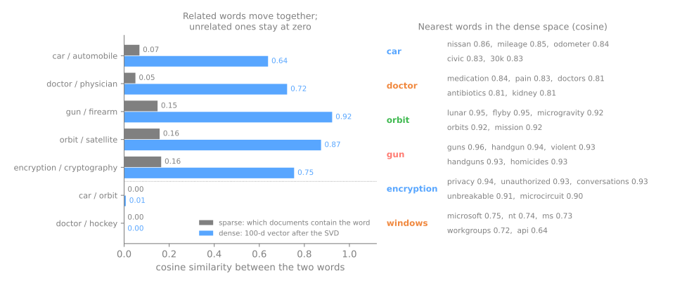
"car" and "automobile" go from 0.07, as TF-IDF columns, to 0.64 as dense vectors; "gun" and "firearm" from 0.15 to 0.92. The control pairs from unrelated subjects stay at 0.00 and 0.01: the SVD did not make everything similar, only words that share contexts. The neighbors also show what kind of similarity a whole post as context produces. "car" is next to nissan, mileage, odometer: words of the same topic, which appear in the same posts. A window of a few words, as in the toy example and in word2vec, produces words of the same kind instead: the nearest words of "car" in GloVe, below, are truck, cars, vehicle.

word2vec: learning vectors by prediction

Skip-gram and CBOW

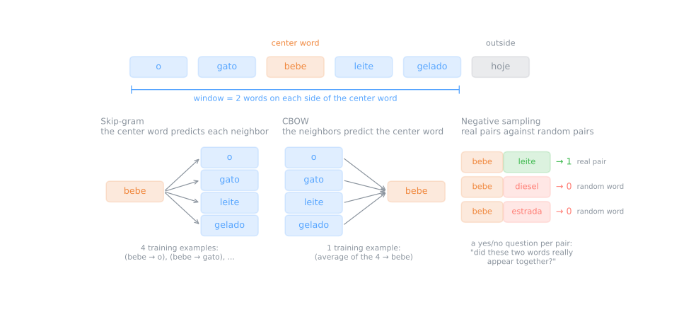
Stage 3. word2vec (Mikolov et al., 2013a) reaches similar vectors by a different road: instead of counting and factorizing, it predicts. It slides a window over the text and turns every position into training examples. The skip-gram variant asks the center word to predict each of its neighbors; the CBOW (continuous bag-of-words) variant asks the neighbors, averaged, to predict the center word:

sentence = "o gato bebe leite gelado hoje".split()     # the cat drinks cold milk today
skipgram = [(sentence[i], sentence[j]) for i in range(len(sentence))
            for j in range(max(0, i - window), min(len(sentence), i + window + 1)) if j != i]
cbow = [([sentence[j] for j in range(max(0, i - window), min(len(sentence), i + window + 1)) if j != i],
         sentence[i]) for i in range(len(sentence))]
print(len(skipgram), 'skip-gram examples (center -> context), e.g.', skipgram[5:9])
print(len(cbow), 'CBOW examples (contexts -> center), e.g.', cbow[2])

18 skip-gram examples (center -> context), e.g. [('bebe', 'o'), ('bebe', 'gato'), ('bebe', 'leite'), ('bebe', 'gelado')]
6 CBOW examples (contexts -> center), e.g. (['o', 'gato', 'leite', 'gelado'], 'bebe')

Every word starts with a random vector of, say, 100 numbers. The model scores a pair (center, context) by the dot product of their vectors, and training nudges the vectors so that pairs that really occur get high scores. The six-word sentence already yields 18 skip-gram examples; a corpus of a billion words yields billions. Words that appear in the same contexts receive the same nudges, so their vectors drift together, which is the distributional hypothesis turned into an optimization.

(figure script)

Negative sampling, in one paragraph

Predicting "which of the 100,000 words of the vocabulary is the neighbor?" would mean computing a score for all 100,000 words at every step. Negative sampling (Mikolov et al., 2013b) replaces it with a much cheaper yes/no question: did these two words really appear together? For each real pair such as (bebe, leite), draw a handful of random words (typically 5 to 20) from the vocabulary and make fake pairs such as (bebe, diesel). The model turns each dot product into a number between 0 and 1 and is trained to answer 1 for the real pair and 0 for the fake ones. Random words are drawn in proportion to their frequency raised to 0.75, so that very common words are not the only negatives. Levy & Goldberg (2014) later showed that skip-gram with negative sampling is, in effect, factorizing a shifted PMI matrix: the prediction road and the counting road of the previous section lead to the same place.

Training word2vec with gensim

The gensim library trains word2vec in one call; the lab does it on one million words of Wikipedia. The parameters are the ones above:

• vector_size: numbers per word (100 to 300 is typical);
• window: how many words on each side count as context. Small windows (2–5) favor words with the same function (other verbs in the same tense); large windows (10+) favor words of the same topic;
• sg=1 for skip-gram, sg=0 for CBOW. Skip-gram is slower and better for rare words; CBOW is faster;
• negative: how many random words per real pair;
• min_count: words rarer than this are dropped (they have too few contexts to learn from);
• epochs: passes over the text; seed and workers=1 make the result reproducible.

GloVe and fastText

Two descendants are worth knowing by name, because their pretrained vectors are everywhere.

GloVe (Pennington, Socher & Manning, 2014), global vectors, goes back to the counting road: it builds the full word–context co-occurrence matrix of a huge corpus and fits vectors whose dot products approximate the logarithm of the counts, with a weight that keeps rare and very frequent pairs from dominating. The Stanford group released vectors trained on 6 billion tokens of Wikipedia and news, which we use below.

fastText (Bojanowski et al., 2017) changes what gets a vector: not the word, but its character n-grams. The vector of a word is the sum of the vectors of its pieces:

def char_ngrams(word, n_min=3, n_max=5):
    w = f"<{word}>"                                  # < and > mark the start and the end
    return [w[i:i + n] for n in range(n_min, n_max + 1) for i in range(len(w) - n + 1)]

print(char_ngrams('latiu'))                           # "barked"
print('shared with "latido":', sorted(set(char_ngrams('latiu')) & set(char_ngrams('latido'))))

['<la', 'lat', 'ati', 'tiu', 'iu>', '<lat', 'lati', 'atiu', 'tiu>', '<lati', 'latiu', 'atiu>']
shared with "latido": ['<la', '<lat', '<lati', 'ati', 'lat', 'lati']

Two consequences. A word never seen in training still gets a vector, built from pieces that other words share: if "latiu" (barked) was never seen but "latido" (a bark) was, six of the pieces are already trained. And inflected forms, which Portuguese has many of (latir, latiu, latia, latindo), share most of their pieces, so they end up close even when some forms are rare. The lab measures both effects, and one side effect: words that are spelled alike but mean different things are pulled together too. fastText also published pretrained vectors for 157 languages, Portuguese included (Grave et al., 2018).

Exploring pretrained vectors

Stage 4. Training good vectors takes billions of words. In practice you download vectors someone else trained. gensim fetches the GloVe vectors trained on 6 billion tokens, in their smallest version (400,000 words, 50 numbers each):

import gensim.downloader as api

glove = api.load('glove-wiki-gigaword-50')     # ~66 MB, downloaded once
print(len(glove.key_to_index), 'words ·', glove.vector_size, 'numbers per word')
print('car =', glove['car'][:6].round(2), '...')
for w in ['car', 'mango', 'doctor', 'brazil', 'python']:
    print(f"{w:7s}", ', '.join(f"{n} {s:.2f}" for n, s in glove.most_similar(w, topn=5)))

400000 words · 50 numbers per word
car = [ 0.48 -0.08  1.46  0.05  0.15  0.51] ...
car     truck 0.92, cars 0.89, vehicle 0.88, driver 0.85, driving 0.84
mango   pineapple 0.91, guava 0.90, papaya 0.89, pear 0.85, coconut 0.85
doctor  nurse 0.80, physician 0.80, patient 0.76, child 0.76, teacher 0.75
brazil  portugal 0.88, argentina 0.87, rica 0.84, spain 0.83, costa 0.83
python  reticulated 0.69, spamalot 0.66, php 0.64, owl 0.63, mouse 0.63

most_similar returns the words with the highest cosine similarity. No single number of the vector means anything ("car" starts with 0.48, −0.08, 1.46, ...); only the geometry does. The neighbors read like a thesaurus built by association: "mango" is surrounded by tropical fruit, "brazil" by other Latin countries (and by "rica" and "costa", the two halves of Costa Rica, because the tokenizer split the name). "python" shows what these vectors learned from: the snake (reticulated), Monty Python (spamalot), and programming languages (php), mixed in one list.

Similar is not synonymous

Cosine similarity measures how interchangeable two words are in context, which is not the same as meaning the same thing:

for a, b in [('car', 'automobile'), ('coffee', 'tea'), ('doctor', 'physician'), ('hot', 'cold'),
             ('good', 'bad'), ('love', 'hate'), ('car', 'banana'), ('doctor', 'guitar')]:
    print(f"{a:6s} / {b:10s} {glove.similarity(a, b):.2f}")

car    / automobile 0.70
coffee / tea        0.81
doctor / physician  0.80
hot    / cold       0.80
good   / bad        0.80
love   / hate       0.65
car    / banana     0.22
doctor / guitar     0.28

Synonyms score high (doctor/physician 0.80), but so do antonyms: hot/cold and good/bad score 0.80, the same as doctor/physician and more than car/automobile (0.70). An antonym is the most interchangeable word there is: "the soup is hot" and "the soup is cold" differ in one word, and every context of one fits the other. The distributional hypothesis measures relatedness, not synonymy. For a search engine this is often fine; for sentiment it is a trap, and the next page measures the same effect on "good" versus "not good".

Analogies, measured honestly

The most famous property of word vectors is that some relations become directions: \(\text{king} - \text{man} + \text{woman}\) lands near \(\text{queen}\) (Mikolov et al., 2013a). most_similar(positive=[a, c], negative=[b]) computes \(a - b + c\) with unit vectors and returns the nearest word. Here are twelve analogies of the kinds used to test word vectors (capitals, verb tenses, comparatives, family, languages), hits and misses alike:

tests = [('king', 'man', 'woman', 'queen'), ('paris', 'france', 'japan', 'tokyo'),
         ('berlin', 'germany', 'italy', 'rome'), ('walked', 'walk', 'swim', 'swam'),
         ('slower', 'slow', 'fast', 'faster'), ('better', 'good', 'bad', 'worse'),
         ('portuguese', 'brazil', 'mexico', 'spanish'), ('bigger', 'big', 'small', 'smaller'),
         ('brother', 'man', 'woman', 'sister'), ('day', 'sun', 'moon', 'night'),
         ('glove', 'hand', 'foot', 'sock'), ('greece', 'athens', 'brasilia', 'brazil')]
hits = 0
for a, b, c, expected in tests:
    got, score = glove.most_similar(positive=[a, c], negative=[b], topn=1)[0]
    hits += got == expected
    print(f"{a:10s} - {b:7s} + {c:8s} = {got:14s} {score:.2f}  "
          f"{'hit' if got == expected else 'miss (expected ' + expected + ')'}")
print(hits, 'hits out of', len(tests))

king       - man     + woman    = queen          0.85  hit
paris      - france  + japan    = tokyo          0.92  hit
berlin     - germany + italy    = rome           0.87  hit
walked     - walk    + swim     = swam           0.80  hit
slower     - slow    + fast     = faster         0.82  hit
better     - good    + bad      = worse          0.90  hit
portuguese - brazil  + mexico   = spanish        0.87  hit
bigger     - big     + small    = larger         0.92  miss (expected smaller)
brother    - man     + woman    = daughter       0.93  miss (expected sister)
day        - sun     + moon     = days           0.74  miss (expected night)
glove      - hand    + foot     = 50,000-square  0.68  miss (expected sock)
greece     - athens  + brasilia = amorim         0.71  miss (expected brazil)
7 hits out of 12

Seven hits out of twelve. Capitals, verb tenses, comparatives and languages mostly work. The misses are instructive:

• bigger − big + small gives larger: the vector found "a comparative" and "a size" but picked the comparative of the wrong adjective;
• brother − man + woman gives daughter, and day − sun + moon gives days: the answer is in the right neighborhood but is not the word you wanted;
• glove − hand + foot and greece − athens + brasilia produce noise ("50,000-square", "amorim"). Relations seen rarely in the training text (Brasília is much rarer than Athens in English news) are not straight directions.

There is also a quiet trick in most_similar: it never returns the input words. Without that rule:

def unit(w):
    return glove.get_vector(w, norm=True)

for a, b, c in [('king', 'man', 'woman'), ('doctor', 'man', 'woman')]:
    v = unit(a) - unit(b) + unit(c)
    print(f"{a} - {b} + {c}, nothing excluded:", ', '.join(f"{w} {s:.2f}" for w, s in glove.similar_by_vector(v, topn=3)))
print(f"cos(king - queen, man - woman) = {cos(unit('king') - unit('queen'), unit('man') - unit('woman')):.2f}")
print(f"cos(king - queen, car - banana) = {cos(unit('king') - unit('queen'), unit('car') - unit('banana')):.2f}")

king - man + woman, nothing excluded: king 0.89, queen 0.85, throne 0.77
doctor - man + woman, nothing excluded: doctor 0.90, nurse 0.84, child 0.77
cos(king - queen, man - woman) = 0.58
cos(king - queen, car - banana) = -0.05

The nearest word to king − man + woman is king itself (0.89); queen is second. Subtracting "man" and adding "woman" moves the vector only a little, and the analogy works because the rule removes the start point. The same rule explains a result often quoted as proof of sexism in embeddings, doctor − man + woman = nurse: the nearest word is doctor (0.90), and "nurse" appears only because "doctor" is forbidden (Nissim, van Noord & van der Goot, 2020). The last two lines measure the "parallel arrows" directly: the offsets king − queen and man − woman have cosine 0.58, clearly related but far from identical, while an unrelated offset scores −0.05. Analogies are a real but approximate regularity, and the lab scores it on thousands of standard questions.

Seeing the space

The simulator below holds the real 50-dimensional GloVe vectors of 143 words. Click a word to see its nearest neighbors, computed in 50 dimensions, drawn as lines on a 2-D map; try the vector arithmetic with the presets (which include misses) and untick "exclude" to see the answer without the rule above. The map can be drawn with PCA or t-SNE, the two projections of dimensionality reduction. The two PCA axes keep only 24.5% of the variance of these vectors, so words that look close on the map may be far apart in 50-D, and vice versa; the lines to the true nearest neighbors show when the projection is lying. t-SNE keeps neighborhoods much better, at the price of distances between groups that mean nothing.

The vectors, the two layouts and the preset answers over the full 400,000-word vocabulary were produced by a short script next to this page (it needs gensim; it rounds each vector to three decimals, which changes no cosine by more than 0.002).

Bias: what the vectors learned about people

Vectors learned from human text absorb the associations of that text, including stereotypes (Bolukbasi et al., 2016; Caliskan, Bryson & Narayanan, 2017). This can be measured without analogies. Average the differences between eight pairs of gendered words (he − she, man − woman, father − mother, ...) to get one gender direction, then project occupation words on it: positive values lean toward "he", negative toward "she".

pairs_gender = [('he', 'she'), ('man', 'woman'), ('father', 'mother'), ('brother', 'sister'),
                ('king', 'queen'), ('boy', 'girl'), ('son', 'daughter'), ('his', 'her')]
g = np.mean([unit(a) - unit(b) for a, b in pairs_gender], axis=0)
g /= np.linalg.norm(g)                   # one "he - she" direction, averaged over 8 pairs
jobs = ['receptionist', 'nurse', 'homemaker', 'hairdresser', 'librarian', 'teacher', 'doctor',
        'accountant', 'carpenter', 'lawyer', 'programmer', 'engineer', 'architect', 'manager', 'captain']
print(pd.Series({w: unit(w) @ g for w in jobs}).sort_values().round(2).to_string())
print('for reference:', {w: round(float(unit(w) @ g), 2) for w in ['she', 'woman', 'man', 'he']})

receptionist   -0.31
homemaker      -0.30
nurse          -0.30
hairdresser    -0.25
librarian      -0.08
teacher         0.00
doctor          0.03
accountant      0.06
carpenter       0.09
lawyer          0.18
programmer      0.19
engineer        0.24
architect       0.32
manager         0.37
captain         0.42
for reference: {'she': -0.19, 'woman': -0.29, 'man': 0.1, 'he': 0.24}

"receptionist", "homemaker" and "nurse" (−0.30) lean further toward "she" than the word "she" itself (−0.19); "manager" (0.37) and "captain" (0.42) lean further toward "he" than "he" (0.24). None of these words is gendered by definition. The vectors did not invent this; they compressed who was written about in which role in Wikipedia and news. Two cautions when reading such a table. The direction is itself estimated from a handful of pairs, and one pair alone can be noisy ("man" is only +0.10 here). And a word can move for reasons unrelated to gender: in news text "captain" is often a sports or military title. What matters in practice is that a system built on these vectors, say one that ranks CVs by similarity to a job description, inherits the lean. Measuring it is the first step; Bolukbasi et al. proposed projecting the direction out, and later work showed that this hides the bias more than it removes it, so it is an open problem, not a solved one.

The limit: one vector per word

Every method on this page gives each word one vector, whatever sense it is used in:

for w in ['bank', 'apple']:
    print(f"{w:6s}", ', '.join(n for n, _ in glove.most_similar(w, topn=10)))
print(f"bank / money {glove.similarity('bank', 'money'):.2f} · bank / river {glove.similarity('bank', 'river'):.2f}")

bank   banks, securities, banking, investment, exchange, financial, credit, lender, capital, brokerage
apple  blackberry, chips, iphone, microsoft, ipad, pc, ipod, intel, ibm, software
bank / money 0.64 · bank / river 0.41

In news text, "bank" is almost always the financial institution, so its single vector is a financial vector: all ten neighbors are about money, and the river bank has vanished (bank/river 0.41 against bank/money 0.64). "apple" is a technology company first and a fruit nowhere in its top ten. A word's vector is roughly a frequency-weighted average of its senses (Arora et al., 2018), dominated by the most frequent one. Portuguese has the same problem with banco (a bank, a bench), manga (a sleeve, a mango) and vela (a candle, a sail).

A second limit follows from the first: a sentence is more than its words. "The dog bit the man" and "the man bit the dog" contain the same words, and any representation built only from word vectors, whatever it does with them, cannot tell who bit whom unless it also looks at order. Both limits are the starting point of sentence embeddings, where the vector of each word is computed from the sentence around it.

Exercises

1. In the toy corpus, compute by hand the co-occurrence row of "caminhão" with window 2, then \(\text{PMI}(\text{caminhão}, \text{diesel})\) using \(N = 126\) and the column total of diesel (count it). Is it larger or smaller than \(\text{PMI}(\text{gato}, \text{bebe}) = 1.81\), and why?
2. With a window of 1 instead of 2, which contexts of "gato" disappear? Would "gato" and "cachorro" still share any context? Predict first, then change window and rerun.
3. In the analogy code, the test bigger − big + small returned "larger". Write two other analogies that you expect to fail for the same reason (the right kind of word, the wrong word), run them, and explain the result.
4. The gender table projects words on a direction built from 8 pairs. Rebuild it from the pair ('he', 'she') alone and compare the position of "man" and "doctor". What does this say about conclusions drawn from a single pair?

Lab: word vectors three ways

The same corpus, three families of vectors, and one fair comparison. The corpus is the first million words of text8, a cleaned dump of English Wikipedia widely used to test word embeddings (Mahoney, 2011): lower-case letters only, numbers spelled out. You will build vectors by counting (PPMI + SVD, as in the toy example), by prediction (word2vec) and download pretrained ones (GloVe), compare their neighbors, score them on a standard analogy test, try fastText on words never seen, and draw the space.

The lab runs in about a minute and a half on a laptop CPU, most of it training word2vec and fastText; the downloads are 31 MB (text8) and 66 MB (GloVe). Run the blocks in order, in one session. To work on it directly, download the lab notebook and open it in Jupyter or Colab (File → Upload notebook); in Colab, run !pip install gensim first.

Step 1 — load a million words of Wikipedia

# In Colab, run once:  !pip install gensim
import numpy as np
import pandas as pd
from collections import Counter
from itertools import islice
import gensim.downloader as api
from gensim.models.word2vec import Text8Corpus

path = api.load('text8', return_path=True)          # 17 million words of Wikipedia, ~31 MB
chunks = list(islice(Text8Corpus(path), 100))       # the first 100 chunks of 10,000 words
tokens = [w for chunk in chunks for w in chunk]
freq = Counter(tokens)
vocab = [w for w, c in freq.most_common() if c >= 10]
pos = {w: i for i, w in enumerate(vocab)}

print(f"{len(tokens):,} tokens · {len(freq):,} distinct words · {len(vocab):,} seen at least 10 times")
print('most frequent:', [w for w, _ in freq.most_common(8)])
print(' '.join(tokens[:22]))

1,000,000 tokens · 52,754 distinct words · 8,412 seen at least 10 times
most frequent: ['the', 'of', 'and', 'one', 'in', 'a', 'to', 'zero']
anarchism originated as a term of abuse first used against early working class radicals including the diggers of the english revolution and

How to read it. The slice has one million tokens and 52,754 distinct words, but only 8,412 appear at least ten times; the rest have too few contexts to learn a vector from, and all three methods drop them (the same min_count=10). The most frequent words are the function words you would expect, plus "one" and "zero", because text8 spells numbers out. (api.load('text8', return_path=True) only downloads the file; reading it with Text8Corpus avoids a loader in the gensim-data package that fails with recent versions of its dependencies.)

Step 2 — count co-occurrences

import scipy.sparse as sp

ids = np.array([pos.get(w, -1) for w in tokens])     # -1 marks a rare word, ignored
rows, cols = [], []
for d in range(1, 5):                                # window: 4 words on each side
    a, b = ids[:-d], ids[d:]
    ok = (a >= 0) & (b >= 0)
    rows += [a[ok], b[ok]]
    cols += [b[ok], a[ok]]                           # count both directions
rows, cols = np.concatenate(rows), np.concatenate(cols)
C = sp.csr_matrix((np.ones(len(rows)), (rows, cols)), shape=(len(vocab), len(vocab)))  # repeats are summed

print(C.shape, f"· {C.nnz:,} non-zero cells ({C.nnz / (C.shape[0] * C.shape[1]):.1%} of the matrix)")
for w, c in [('king', 'queen'), ('king', 'the'), ('king', 'car')]:
    print(f"count({w}, {c}) = {int(C[pos[w], pos[c]])}")

(8412, 8412) · 1,740,671 non-zero cells (2.5% of the matrix)
count(king, queen) = 7
count(king, the) = 321
count(king, car) = 0

How to read it. This is the toy example at scale, written without Python loops: for each distance d from 1 to 4, the arrays ids[:-d] and ids[d:] line up every word with the word d positions later, and each aligned pair is one co-occurrence. The matrix has 8,412 × 8,412 cells, about 71 million, and only 2.5% are non-zero: most pairs of words never meet within four positions, so it is stored sparse, like the bag-of-words matrices. "king" meets "the" far more often than "queen", which is exactly the imbalance PPMI corrects.

Step 3 — PPMI and SVD

from sklearn.decomposition import TruncatedSVD
from sklearn.preprocessing import normalize

N = C.sum()
n_word = np.asarray(C.sum(axis=1)).ravel()
n_ctx = np.asarray(C.sum(axis=0)).ravel()
Cc = C.tocoo()
pmi = np.log2(Cc.data * N / (n_word[Cc.row] * n_ctx[Cc.col]))   # only the non-zero cells
keep = pmi > 0
PPMI = sp.csr_matrix((pmi[keep], (Cc.row[keep], Cc.col[keep])), shape=C.shape)
W_svd = normalize(TruncatedSVD(n_components=100, random_state=0).fit_transform(PPMI))

def neighbors(W, word, k=6):
    sims = W @ W[pos[word]]                          # rows have length 1: dot = cosine
    best = [j for j in np.argsort(-sims) if j != pos[word]][:k]
    return ', '.join(vocab[j] for j in best)

probe = ['king', 'car', 'france', 'computer', 'bank', 'four']
print(f"{PPMI.nnz:,} positive PPMI cells of {C.nnz:,} · word vectors {W_svd.shape}")
for w in probe:
    print(f"{w:9s}", neighbors(W_svd, w))

1,508,032 positive PPMI cells of 1,740,671 · word vectors (8412, 100)
king      ii, alexander, son, iv, queen, iii
car       racing, audi, cars, touring, auto, wheel
france    spain, portugal, netherlands, norway, kingdom, brazil
computer  computers, software, portable, hardware, digital, apple
bank      caribbean, eastern, country, western, settlement, nations
four      six, five, three, seven, two, eight

How to read it. PMI is computed only on the non-zero cells (a zero count would give \(-\infty\), which PPMI clips to 0 anyway), and 87% of them are positive. The SVD compresses each word's 8,412 PPMI values to 100 numbers, and normalize gives every vector length 1, so a dot product is a cosine. The neighbors are sensible for a method that took seconds: numbers next to numbers, countries next to countries, "computer" next to "software" and "hardware". "king" is surrounded by regnal numbers (ii, iv, iii), because in Wikipedia kings are followed by them. "bank" is the weak one: its neighbors are geographic (caribbean, eastern, western), because in this slice "bank" is often the West Bank or a river bank, and one vector has to cover them all.

Step 4 — word2vec on the same text

from gensim.models import Word2Vec

w2v = Word2Vec(chunks, vector_size=100, window=4, min_count=10, sg=1, negative=5,
               epochs=5, workers=1, seed=0)          # sg=1: skip-gram · workers=1 + seed: reproducible
W_w2v = normalize(np.array([w2v.wv[w] for w in vocab]))
print(len(w2v.wv), 'words ·', w2v.wv.vector_size, 'numbers each')
for w in probe:
    print(f"{w:9s}", neighbors(W_w2v, w))

8412 words · 100 numbers each
king      queen, philip, pope, khan, duke, son
car       racing, touring, driver, automobile, sports, radio
france    spain, portugal, norway, archbishop, brazil, canterbury
computer  macintosh, software, animation, video, computing, newton
bank      continental, luanda, jutland, reef, northwestern, bering
four      three, five, six, seven, eight, one

How to read it. The same vocabulary (8,412 words, thanks to min_count=10), the same window, the same size of vector, so the comparison is fair. word2vec gets "king" right where counting did not (queen, then philip, pope, khan, duke: other rulers), and puts "automobile" among the neighbors of "car". It also makes odd choices: "archbishop" and "canterbury" next to "france", and for "bank" a list of places (luanda, jutland, reef, bering). With only one million words, each of these is decided by a few dozen contexts. workers=1 matters: with several threads the order of the updates changes from run to run, and so do the vectors.

Step 5 — pretrained GloVe

glove = api.load('glove-wiki-gigaword-50')          # trained on 6 billion tokens, ~66 MB
known = [w in glove.key_to_index for w in vocab]
W_glove = normalize(np.array([glove[w] if k else np.zeros(50) for w, k in zip(vocab, known)]))
print(f"{sum(known):,} of our {len(vocab):,} words are in GloVe")
for w in probe:
    print(f"{w:9s}", neighbors(W_glove, w))

8,383 of our 8,412 words are in GloVe
king      prince, queen, ii, emperor, son, uncle
car       cars, vehicle, driver, driving, bus, vehicles
france    french, belgium, paris, spain, netherlands, italy
computer  computers, software, technology, electronic, internet, computing
bank      banks, banking, investment, exchange, financial, credit
four      three, six, five, eight, seven, two

How to read it. To compare like with like, the GloVe vectors are restricted to our 8,412 words (29 of them, like odd spellings, are missing and get a zero vector). The neighbors are now uniformly good: "car" → cars, vehicle, driver; "france" → french, belgium, paris; "bank" → banks, banking, investment. GloVe has half as many numbers per word (50 against 100), and it wins anyway, because it saw 6,000 times more text. With word vectors, the amount of training text matters more than the choice of algorithm.

Step 6 — the analogy test: 3,732 questions

from gensim.test.utils import datapath

questions, section = [], None
for line in open(datapath('questions-words.txt')):   # Mikolov et al.'s analogy test set
    if line.startswith(':'):
        section = 'syntactic' if line.startswith(': gram') else 'semantic'
        continue
    q = line.lower().split()
    if all(w in pos and w in glove.key_to_index for w in q):
        questions.append((section, *q))
print(len(questions), 'questions use only words that all three models know:',
      dict(Counter(s for s, *_ in questions)))

def analogy_accuracy(W):
    hits = Counter()
    for section, a, b, c, d in questions:            # "a is to b as c is to d": b - a + c ≈ d
        sims = W @ (W[pos[b]] - W[pos[a]] + W[pos[c]])
        sims[[pos[a], pos[b], pos[c]]] = -np.inf     # the usual rule: inputs cannot be the answer
        hits[section] += vocab[np.argmax(sims)] == d
    n = Counter(s for s, *_ in questions)
    return {s: hits[s] / n[s] for s in ['semantic', 'syntactic']} | {'all': sum(hits.values()) / len(questions)}

print(pd.DataFrame({'PPMI + SVD': analogy_accuracy(W_svd), 'word2vec': analogy_accuracy(W_w2v),
                    'GloVe (pretrained)': analogy_accuracy(W_glove)}).T.round(3))

3732 questions use only words that all three models know: {'semantic': 418, 'syntactic': 3314}
                    semantic  syntactic    all
PPMI + SVD             0.287      0.099  0.120
word2vec               0.153      0.050  0.062
GloVe (pretrained)     0.722      0.585  0.600

How to read it. questions-words.txt ships with gensim: the analogy questions of Mikolov et al. (2013a), such as athens greece baghdad iraq (semantic: capitals, currencies, family) and walk walking swim swimming (syntactic: tenses, plurals, comparatives). We keep the 3,732 questions whose four words are in our vocabulary and in GloVe, and every model searches the same 8,412 candidates, so the scores are comparable. A random guess would score about 0.01%.

• GloVe answers 60.0% correctly (72.2% semantic). That is the number behind the famous examples: impressive, and also wrong four times in ten.
• PPMI + SVD scores 12.0%, word2vec 6.2%. On one million words, the counting method beats the predicting one, in line with Levy, Goldberg & Dagan (2015), who found that with the same data and comparable settings neither family is systematically better. word2vec's advantage in the original papers came with billions of words and careful tuning.
• Semantic questions are easier for all three here, because many of them are capitals and countries, which Wikipedia mentions together constantly.

Step 7 — a word never seen: fastText

from gensim.models import FastText

ft = FastText(chunks, vector_size=100, window=4, min_count=10, sg=1, epochs=5,
              bucket=200_000, workers=1, seed=0)
for w in ['computers', 'compuetr', 'microcomputers', 'unhappyness', 'cattle']:
    status = 'in vocabulary' if w in ft.wv.key_to_index else 'never seen   '
    print(f"{w:15s} {status}  ", ', '.join(n for n, _ in ft.wv.most_similar(w, topn=4)))
print('does word2vec know "compuetr"?', 'compuetr' in w2v.wv.key_to_index)

computers       in vocabulary   computer, programmers, programs, computing
compuetr        never seen      computer, computing, compact, computers
microcomputers  never seen      computers, programmers, computer, machines
unhappyness     never seen      sickness, illness, happiness, predecessor
cattle          in vocabulary   bottle, wattle, battle, battles
does word2vec know "compuetr"? False

How to read it. fastText trains on the same text, but learns vectors for character n-grams (bucket is the size of the table that holds them). The misspelling "compuetr" and the rare "microcomputers" were never seen, yet their vectors, assembled from pieces, land next to "computer" and "computers"; word2vec has no vector for them at all. The two last rows show the price. "unhappyness" gets "happiness" but also "sickness" and "illness", which share the suffix -ness. And "cattle", a word it has seen, gets bottle, wattle, battle: spelling neighbors, not meaning neighbors. On a small corpus the n-grams speak louder than the contexts.

Step 8 — draw the space

import matplotlib.pyplot as plt
from sklearn.decomposition import PCA
from sklearn.manifold import TSNE

words = ['king', 'queen', 'man', 'woman', 'prince', 'princess', 'paris', 'france', 'rome', 'italy',
         'tokyo', 'japan', 'berlin', 'germany', 'car', 'truck', 'bus', 'train', 'dog', 'cat', 'horse',
         'cow', 'apple', 'banana', 'mango', 'orange', 'walk', 'walked', 'swim', 'swam', 'run', 'ran']
X = np.array([glove.get_vector(w, norm=True) for w in words])
pca = PCA(n_components=2).fit(X)
maps = {'PCA': pca.transform(X),
        't-SNE': TSNE(n_components=2, perplexity=8, metric='cosine', init='pca',
                      random_state=0).fit_transform(X)}
print(f"PCA: the 2 axes keep {pca.explained_variance_ratio_.sum():.0%} of the variance of these {len(words)} vectors")

fig, axes = plt.subplots(1, 2, figsize=(12, 5))
for ax, (name, P) in zip(axes, maps.items()):
    ax.scatter(P[:, 0], P[:, 1], s=12)
    for w, (x, y) in zip(words, P):
        ax.annotate(w, (x, y), fontsize=8)
    ax.set_title(f'GloVe vectors, {name}')
plt.show()

PCA: the 2 axes keep 36% of the variance of these 32 vectors

How to read it. The two PCA axes keep 36% of the variance of these 32 vectors, so the PCA map is a rough shadow: the groups (royalty, capitals and countries, vehicles, animals, fruit, verbs) are visible but overlap. The t-SNE map separates them cleanly, because it only tries to keep each word next to its nearest neighbors. Look for the pairs: in both maps each capital sits near its country, and the offsets country → capital point in roughly similar directions, which is the analogy regularity seen in 2-D. Remember the lesson of dimensionality reduction: distances between t-SNE groups mean nothing, so "fruit is far from verbs" is not a finding.

Your turn

1. Window size. Retrain word2vec (step 4) with window=2 and with window=10, and compare the neighbors of "walked", "computer" and "france". Which window gives neighbors of the same grammatical kind, and which gives neighbors of the same topic?
2. More text. Change the 100 chunks of step 1 to 300 (three million words) and rerun steps 1 to 6. How much do the analogy scores of PPMI + SVD and word2vec change? Is the gap to GloVe closing?
3. Bias in your own list. Using the gender direction from the page, project fifteen words of your choice (sports, adjectives such as "brilliant" and "beautiful", names) on it with the GloVe vectors. Which results surprise you? Build a second direction from ('rich', 'poor') and repeat.
4. A thesaurus from counts. Use neighbors(W_svd, ...) to find three words for which PPMI + SVD gives better neighbors than word2vec, and three for which it gives worse ones. Can you see a pattern in word frequency?

Class materials

References

• Harris, Z. S. "Distributional Structure." Word 10, no. 2–3 (1954): 146–162 — the distributional hypothesis. DOI
• Firth, J. R. "A Synopsis of Linguistic Theory, 1930–1955." In Studies in Linguistic Analysis, 1–32. Oxford: Blackwell (1957) — "You shall know a word by the company it keeps."
• Church, K. W.; Hanks, P. "Word Association Norms, Mutual Information, and Lexicography." Computational Linguistics 16, no. 1 (1990): 22–29 — pointwise mutual information for word pairs. ACL Anthology
• Deerwester, S.; Dumais, S. T.; Furnas, G. W.; Landauer, T. K.; Harshman, R. "Indexing by Latent Semantic Analysis." Journal of the American Society for Information Science 41, no. 6 (1990): 391–407 — the SVD of the term–document matrix. DOI
• Mikolov, T.; Chen, K.; Corrado, G.; Dean, J. "Efficient Estimation of Word Representations in Vector Space." ICLR Workshop (2013) — word2vec (skip-gram and CBOW) and the analogy test set. arXiv:1301.3781
• Mikolov, T.; Sutskever, I.; Chen, K.; Corrado, G.; Dean, J. "Distributed Representations of Words and Phrases and their Compositionality." NeurIPS 26 (2013): 3111–3119 — negative sampling. arXiv:1310.4546
• Levy, O.; Goldberg, Y. "Neural Word Embedding as Implicit Matrix Factorization." NeurIPS 27 (2014): 2177–2185 — skip-gram with negative sampling factorizes a shifted PMI matrix. Proceedings
• Levy, O.; Goldberg, Y.; Dagan, I. "Improving Distributional Similarity with Lessons Learned from Word Embeddings." TACL 3 (2015): 211–225 — count-based and prediction-based vectors compared on equal terms. DOI
• Pennington, J.; Socher, R.; Manning, C. D. "GloVe: Global Vectors for Word Representation." EMNLP (2014): 1532–1543. DOI
• Bojanowski, P.; Grave, E.; Joulin, A.; Mikolov, T. "Enriching Word Vectors with Subword Information." TACL 5 (2017): 135–146 — fastText. DOI
• Grave, E.; Bojanowski, P.; Gupta, P.; Joulin, A.; Mikolov, T. "Learning Word Vectors for 157 Languages." LREC (2018) — pretrained fastText vectors, Portuguese included. arXiv:1802.06893
• Bolukbasi, T.; Chang, K.-W.; Zou, J.; Saligrama, V.; Kalai, A. "Man is to Computer Programmer as Woman is to Homemaker? Debiasing Word Embeddings." NeurIPS 29 (2016): 4349–4357. arXiv:1607.06520
• Caliskan, A.; Bryson, J. J.; Narayanan, A. "Semantics Derived Automatically from Language Corpora Contain Human-like Biases." Science 356, no. 6334 (2017): 183–186. DOI
• Nissim, M.; van Noord, R.; van der Goot, R. "Fair Is Better than Sensational: Man Is to Doctor as Woman Is to Doctor." Computational Linguistics 46, no. 2 (2020): 487–497 — how the exclusion rule shapes analogy results. DOI
• Arora, S.; Li, Y.; Liang, Y.; Ma, T.; Risteski, A. "Linear Algebraic Structure of Word Senses, with Applications to Polysemy." TACL 6 (2018): 483–495 — a word's vector as a weighted mix of its senses. DOI
• Mahoney, M. "About the Test Data." Large Text Compression Benchmark (2011) — text8, the first 10⁸ bytes of the English Wikipedia dump of March 2006, cleaned. mattmahoney.net/dc/textdata.html
• Jurafsky, D.; Martin, J. H. Speech and Language Processing, 3rd ed. draft, chapter 6 "Vector Semantics and Embeddings" — PPMI, word2vec and bias, at textbook pace. Full text

Quiz