The problem: every word is its own column
- In bag-of-words and TF-IDF the columns are orthogonal.
- "car" and "automobile" are exactly as unrelated as "car" and "banana".
- The representation knows which words a document contains, nothing about what they mean.
The path of this lesson
- Context → meaningthe distributional hypothesis
- Count and compressco-occurrence counts → PPMI → truncated SVD
- Learn by predictingword2vec, GloVe, fastText
- Explore the spaceneighbors, analogies, bias, one vector per word
A word you have never seen
- Um copo de tiquira gelada. (A glass of cold tiquira.)
- A tiquira é feita de mandioca fermentada. (… made from fermented cassava.)
- Bebeu tiquira demais e passou mal. (He drank too much … and felt sick.)
- No Maranhão, servem tiquira nas festas. (… they serve it at parties.)
The distributional hypothesis
You inferred it from the company it keeps: glass, cold, fermented, drank, too much, parties.
Harris, 1954
words that occur in similar contexts tend to have similar meanings
Firth, 1957
"you shall know a word by the company it keeps"
A toy corpus: 11 sentences
animals
o gato bebe leite · o gato come peixe · o cachorro bebe água · o cachorro come carne · o cachorro corre na rua
vehicles
o carro usa gasolina · o carro corre na estrada · o automóvel usa gasolina · o automóvel anda na estrada · o caminhão usa diesel · o caminhão corre na estrada
Designed so that gato/cachorro and carro/automóvel never share a sentence, but share their neighbors.
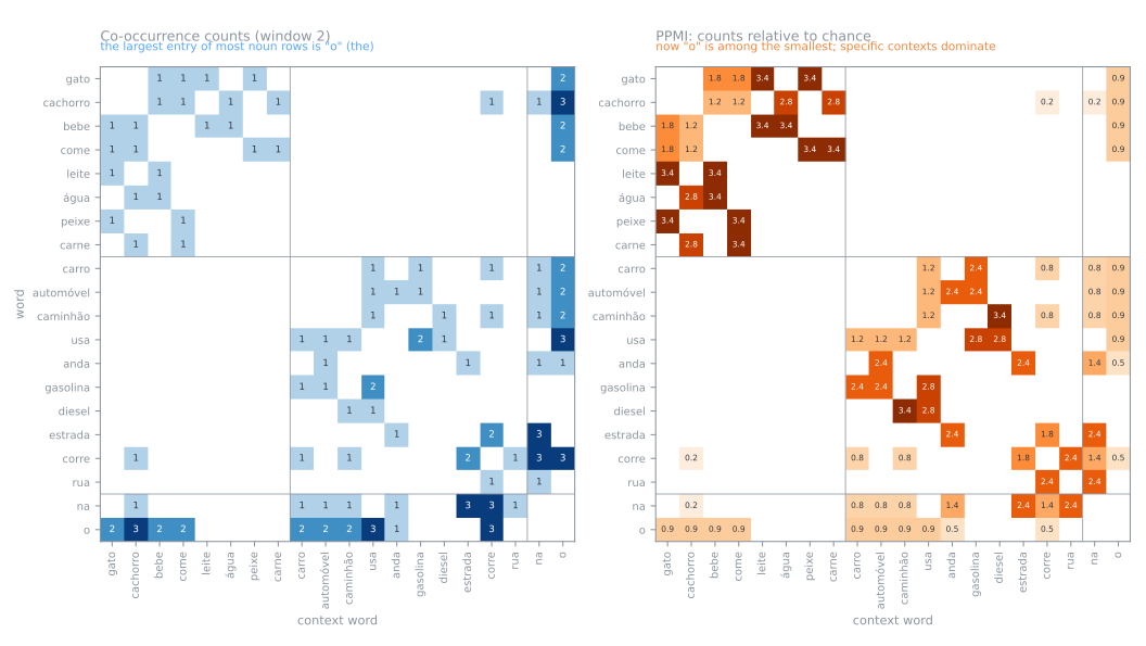
For each word, count every other word within a window of two words to the left or right: a 20 × 20 matrix, 126 (word, context) pairs.
One row by hand: "gato"
- "o gato bebe leite": the window holds o, bebe, leite.
- "o gato come peixe": the window holds o, come, peixe.
| word | its row: the context profile |
|---|---|
| gato | bebe 1 · come 1 · leite 1 · o 2 · peixe 1 |
| cachorro | bebe 1 · carne 1 · come 1 · corre 1 · na 1 · o 3 · água 1 |
| carro | corre 1 · gasolina 1 · na 1 · o 2 · usa 1 |
| automóvel | anda 1 · gasolina 1 · na 1 · o 2 · usa 1 |
Documents versus contexts
| pair | bag-of-words columns | co-occurrence rows |
|---|---|---|
| gato / cachorro | 0.00 | 0.73 |
| carro / automóvel | 0.00 | 0.87 |
| gato / carro | 0.00 | 0.50 |
PMI: counting what is surprising
Not "how often together?" but "how much more often than chance?" (Church & Hanks, 1990)
\[ \text{PMI}(w, c) = \log_2 \frac{P(w, c)}{P(w)\,P(c)} = \log_2 \frac{n(w, c) \cdot N}{n(w) \cdot n(c)} \]PMI(gato, bebe)
\(\log_2 \frac{1 \times 126}{6 \times 6}\)
PMI(gato, o)
\(\log_2 \frac{2 \times 126}{6 \times 22}\)
o is next to everything (22 times as a context): barely surprising. The order of the raw counts flips. Clip negatives to zero: PPMI \(= \max(\text{PMI}, 0)\).
PPMI fixes the article, and becomes too literal
| pair | counts | PPMI |
|---|---|---|
| gato / cachorro | 0.73 | 0.22 |
| carro / automóvel | 0.87 | 0.75 |
| gato / carro | 0.50 | 0.05 |
Cat and dog share only bebe and come: milk, water, fish, meat are four orthogonal columns.
Truncated SVD: 20 sparse columns → 2 dense numbers
| word | dim 1 | dim 2 |
|---|---|---|
| gato | 3.77 | −0.97 |
| cachorro | 2.55 | −0.35 |
| leite | 2.78 | −0.79 |
| carro | 0.61 | 1.87 |
| automóvel | 0.70 | 2.28 |
| gasolina | 0.64 | 2.44 |
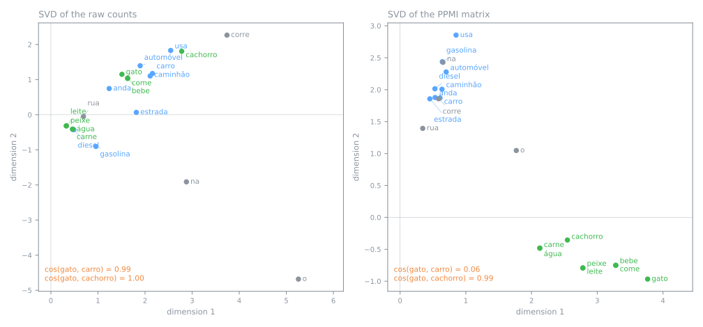
The SVD (PCA without centering) keeps the \(k\) directions that explain most of the matrix.
Animals and food: big first coordinate. Vehicles and fuel: big second.
The whole section in four columns
| pair | BoW columns | counts | PPMI | PPMI + SVD |
|---|---|---|---|---|
| gato / cachorro | 0.00 | 0.73 | 0.22 | 0.99 |
| carro / automóvel | 0.00 | 0.87 | 0.75 | 1.00 |
| gato / carro | 0.00 | 0.50 | 0.05 | 0.06 |
The same compression on documents: LSA
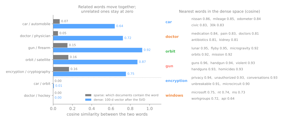
Latent semantic analysis (LSA, Deerwester et al., 1990): truncated SVD of the TF-IDF matrix, 11,314 posts, 100 components.
car/automobile 0.07 → 0.64; gun/firearm 0.15 → 0.92; unrelated pairs stay at 0.00–0.01.
word2vec: learning by prediction
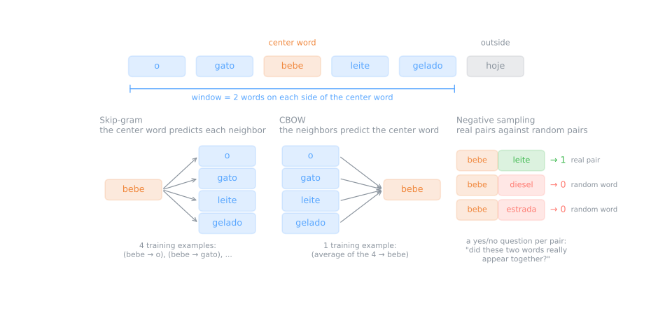
Mikolov et al., 2013. Slide a window and make training examples:
- skip-gram: the center predicts each neighbor → 18 examples from 6 words;
- CBOW: the averaged neighbors predict the center → 6 examples.
How the vectors drift together
- Every word starts with a random vector. A pair (center, context) is scored by the dot product.
- Training nudges the vectors so that pairs that really occur score high.
- Words in the same contexts get the same nudges: the distributional hypothesis as an optimization.
negative sampling
Instead of scoring all 100,000 words: "did these two really appear together?" Real (bebe, leite) → 1; random (bebe, diesel) → 0, with 5 to 20 random words per real pair.
Training it: the knobs of gensim
| parameter | what it does |
|---|---|
vector_size | numbers per word (100 to 300 is typical) |
window | small (2–5): same function; large (10+): same topic |
sg | 1 = skip-gram (slower, better for rare words); 0 = CBOW |
negative | random words per real pair |
min_count | rarer words are dropped |
epochs, seed | passes; seed and workers=1 for reproducibility |
GloVe and fastText
GloVe (Pennington et al., 2014)
Back to counting: fit vectors whose dot products approximate the log of the co-occurrence counts of a huge corpus.
fastText (Bojanowski et al., 2017)
A word is the sum of its character n-grams:
latiu → <la, lat, ati, tiu, iu>, <lat, lati, …
6 pieces shared with latido
Pretrained vectors: GloVe, 400,000 words × 50 numbers
| word | nearest by cosine |
|---|---|
| car | truck 0.92, cars 0.89, vehicle 0.88, driver 0.85, driving 0.84 |
| mango | pineapple 0.91, guava 0.90, papaya 0.89, pear 0.85, coconut 0.85 |
| brazil | portugal 0.88, argentina 0.87, rica 0.84, spain 0.83, costa 0.83 |
| python | reticulated 0.69, spamalot 0.66, php 0.64, owl 0.63, mouse 0.63 |
No single number means anything ("car" starts with 0.48, −0.08, 1.46…); only the geometry does. "python" mixes the snake, Monty Python and programming.
Similar is not synonymous
| car / automobile | 0.70 |
| doctor / physician | 0.80 |
| hot / cold | 0.80 |
| good / bad | 0.80 |
| car / banana | 0.22 |
An antonym is the most interchangeable word there is: "the soup is hot" / "the soup is cold".
Analogies, measured honestly
\(\text{king} - \text{man} + \text{woman} \approx\ ?\)
hits
queen · tokyo · rome · swam · faster · worse · spanish
misses
- bigger − big + small = larger
- brother − man + woman = daughter
- glove − hand + foot = "50,000-square"
Capitals, tenses, comparatives and languages mostly work; rare relations are not straight directions.
The quiet trick: the input words are excluded
| nothing excluded | nearest three |
|---|---|
| king − man + woman | king 0.89, queen 0.85, throne 0.77 |
| doctor − man + woman | doctor 0.90, nurse 0.84, child 0.77 |
- "doctor − man + woman = nurse" appears only because "doctor" is forbidden (Nissim et al., 2020).
- cos(king − queen, man − woman) = 0.58; an unrelated offset: −0.05.
Simulator: seeing the space
Predict. Click a word and compare its neighbors in 50-D (the lines) with the map: does the PCA map (24.5% of the variance) lie? Then untick "exclude".
Bias: what the vectors learned about people
Average 8 differences (he − she, man − woman, …) into a gender direction; project occupations on it.
| receptionist | −0.31 |
| nurse | −0.30 |
| teacher | 0.00 |
| engineer | 0.24 |
| manager | 0.37 |
| captain | 0.42 |
For reference: she −0.19, he 0.24. Receptionist leans further to "she" than "she"; captain further to "he" than "he".
The limit: one vector per word
bank
banks, securities, banking, investment, exchange, financial…
bank/money 0.64 · bank/river 0.41
apple
blackberry, chips, iphone, microsoft, ipad…
the fruit is nowhere in the top ten
- A vector is roughly a frequency-weighted average of the senses (Arora et al., 2018). Portuguese: banco, manga, vela.
- "The dog bit the man" / "the man bit the dog": same words, so word vectors alone cannot tell who bit whom.
Summary
- Distributional hypothesis: similar contexts → similar vectors.
- By hand: co-occurrence counts → PPMI (remove the obvious) → SVD (generalize).
- word2vec predicts neighbors; it lands near the same place as counting. fastText uses pieces of words.
- Pretrained vectors: neighbors, relatedness (antonyms too), approximate analogies, absorbed bias.
- One vector per word, whatever the sense.
Word vectors three ways
- The first million words of text8 (English Wikipedia, cleaned).
- Counting (PPMI + SVD), prediction (word2vec) and pretrained (GloVe): neighbors, the analogy test (3,732 questions), fastText on words never seen, a map of the space.
- Download the lab notebook and open it in Jupyter or Colab; in Colab run
!pip install gensimfirst. - Run the blocks in order and compare with the outputs on the page.
Downloads: 31 MB (text8) and 66 MB (GloVe).