U5.3 BERTopic

BERTopic takes the second answer of What is a topic?: a topic is a cluster of documents. This page first measures why that helps, on short documents where word counts run out; then it runs BERTopic's four steps one at a time on the 2,155 posts, checks that the BERTopic class does exactly the same in one call, and tunes the topic words afterwards.

import numpy as np
import pandas as pd
from sklearn.feature_extraction.text import CountVectorizer

docs_toy = [
    "the team won the game with a late goal",                 # sports
    "fans cheered when the team scored a goal",
    "the coach said the game was a fair win for the team",
    "the rocket launch put a satellite in orbit",             # space
    "nasa delayed the rocket launch to the moon",
    "the satellite reached orbit around the moon",
    "bake the bread in a hot oven",                           # cooking
    "knead the dough and bake the bread slowly",
    "fresh bread from the oven smells great",
    "the team watched the rocket launch before the game",     # sports + space
    "astronauts ate fresh bread on the moon",                 # space + cooking
]

def top_words(components, vocab, n=4):
    return [' '.join(vocab[row.argsort()[::-1][:n]]) for row in components]

from sklearn.datasets import fetch_20newsgroups

forums = ['comp.graphics', 'rec.sport.hockey', 'sci.space', 'soc.religion.christian']
ng = fetch_20newsgroups(subset='train', categories=forums, random_state=0,
                        remove=('headers', 'footers', 'quotes'))   # keep only the body text
long_enough = np.array([len(text.split()) >= 20 for text in ng.data])
docs = [text for text, keep in zip(ng.data, long_enough) if keep]
y = ng.target[long_enough]                                         # the forum: used only to check

from sklearn.metrics import adjusted_rand_score

settings = dict(stop_words='english', min_df=5, max_df=0.5,
                token_pattern=r'(?u)\b[a-zA-Z]{3,}\b')             # words of 3+ letters, no numbers
cv = CountVectorizer(**settings)
X = cv.fit_transform(docs)
vocab = cv.get_feature_names_out()

from sklearn.decomposition import NMF
from sklearn.feature_extraction.text import TfidfVectorizer

tv = TfidfVectorizer(**settings)
T = tv.fit_transform(docs)                                  # same vocabulary as X, TF-IDF weights

Short documents: where word counts run out

Stage 4. LDA and NMF see a document only through its word counts. A tweet, a review title or a support-ticket subject has five to twenty words, so two documents on the same subject often share none. To measure how much this matters, cut every post of the corpus to its first \(n\) words and fit both models again (figure script):

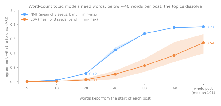
With the first 20 words, both models are close to chance: ARI 0.12 for NMF and 0.03 for LDA. A sentence embedding does not need shared words, because it was trained on huge amounts of text to place sentences with the same meaning close together:

from sklearn.cluster import KMeans
from sklearn.metrics.pairwise import cosine_similarity
from sentence_transformers import SentenceTransformer

pair = ["I want my money back", "please process a refund"]
print(f"TF-IDF cosine:    {cosine_similarity(TfidfVectorizer().fit_transform(pair))[0, 1]:.2f}")
encoder = SentenceTransformer('all-MiniLM-L6-v2')
print(f"embedding cosine: {cosine_similarity(encoder.encode(pair))[0, 1]:.2f}")

short = [' '.join(text.split()[:20]) for text in docs]           # keep the first 20 words only
T_short = TfidfVectorizer(**{**settings, 'min_df': 2}).fit_transform(short)
nmf_short = NMF(n_components=4, init='nndsvda', max_iter=500,
                random_state=0).fit_transform(T_short).argmax(axis=1)
E_short = encoder.encode(short, show_progress_bar=False)
km_short = KMeans(n_clusters=4, n_init=10, random_state=0).fit_predict(E_short)
print(f"first 20 words only -> ARI  NMF on TF-IDF {adjusted_rand_score(y, nmf_short):.3f}"
      f"   k-means on embeddings {adjusted_rand_score(y, km_short):.3f}")

TF-IDF cosine:    0.00
embedding cosine: 0.60
first 20 words only -> ARI  NMF on TF-IDF 0.115   k-means on embeddings 0.582

The two refund requests share no word, so their TF-IDF vectors are orthogonal (cosine 0); their embeddings have a cosine of 0.60. On the 20-word posts, plain k-means on the embeddings reaches an ARI of 0.582, five times NMF's. This is the idea behind BERTopic: first place the documents where meaning is distance, then look for groups.

BERTopic: topics as clusters of documents

BERTopic (Grootendorst, 2022) replaces the generative story with a geometric one: embed the documents so that similar meaning becomes spatial proximity, find the dense regions, and describe each region by its words. It is a chain of four independent steps, and each one is a lesson you have already seen:

This section runs the steps one at a time on the 2,155 posts and inspects the output of each, then shows that BERTopic does exactly the same in one call. Outside this site, install it with pip install bertopic (in Colab too); it brings sentence-transformers, umap-learn and hdbscan with it.

Step 1 — embed

from sklearn.neighbors import NearestNeighbors

E = encoder.encode(docs, show_progress_bar=False)       # stage 1: one 384-d vector per post
print(E.shape)

def same_forum_neighbors(V, metric, k=10):             # share of each post's k nearest posts
    nn = NearestNeighbors(n_neighbors=k + 1, metric=metric).fit(V)   # from the same forum
    idx = nn.kneighbors(V, return_distance=False)[:, 1:]
    return (y[idx] == y[:, None]).mean()

print(f"10 nearest neighbors in the same forum:  TF-IDF {same_forum_neighbors(T, 'cosine'):.3f}"
      f"   embeddings {same_forum_neighbors(E, 'cosine'):.3f}")

(2155, 384)
10 nearest neighbors in the same forum:  TF-IDF 0.832   embeddings 0.942

all-MiniLM-L6-v2 is a small sentence-transformer (Reimers & Gurevych, 2019): 384 dimensions, fast on a CPU, trained on English. It reads only the first 256 word pieces of each post, which is enough here. A quick check that the space is useful before clustering in it: for each post, take its 10 nearest posts and count how many come from the same forum. With TF-IDF vectors, 83.2%; with embeddings, 94.2%.

Step 2 — reduce with UMAP

Density-based clustering suffers in 384 dimensions: distances concentrate, and every point looks about as far from every other (the curse of dimensionality). BERTopic first compresses the embeddings with UMAP (McInnes, Healy & Melville, 2018), which keeps each point's neighborhood:

from umap import UMAP

umap_model = UMAP(n_neighbors=15, n_components=5, min_dist=0.0, metric='cosine',
                  random_state=42)                      # BERTopic's defaults, plus a seed
Z = umap_model.fit_transform(E)                         # stage 2: 384 -> 5 dimensions
print(Z.shape)
print(f"10 nearest neighbors in the same forum after UMAP: {same_forum_neighbors(Z, 'euclidean'):.3f}")

(2155, 5)
10 nearest neighbors in the same forum after UMAP: 0.954

Five dimensions, not two: the goal is to cluster, not to draw, and two dimensions would squeeze too much. min_dist=0.0 lets UMAP pack similar points tightly, which is what a density-based clusterer wants. The neighborhoods survived the compression (95.4% of neighbors from the same forum, slightly more than in 384 dimensions). UMAP is stochastic; random_state makes it repeatable, a point the pitfalls come back to.

Step 3 — cluster with HDBSCAN; outliers are topic −1

HDBSCAN (Campello, Moulavi & Sander, 2013) finds dense regions of any shape and density, with one main knob, min_cluster_size. Two of its properties matter here: the number of clusters comes out of the data, and it does not force every point into a cluster: points in sparse regions get the label −1. BERTopic uses the hdbscan package, the same algorithm as sklearn.cluster.HDBSCAN from the clustering lesson in a different implementation:

from hdbscan import HDBSCAN

hdbscan_model = HDBSCAN(min_cluster_size=10, metric='euclidean',
                        cluster_selection_method='eom', prediction_data=True)
labels = hdbscan_model.fit_predict(Z)                   # stage 3: dense regions; -1 = outlier
n_clusters = labels.max() + 1
print(n_clusters, 'clusters |', (labels == -1).sum(), f'outliers ({(labels == -1).mean():.1%})')

tab = pd.crosstab(labels, np.array(forums)[y], rownames=['cluster'], colnames=['forum'])
share = (tab.max(axis=1) / tab.sum(axis=1)).drop(-1)   # share of the majority forum per cluster
print(f"clusters whose majority forum holds at least 90% of the posts: {(share >= 0.9).sum()} of {n_clusters}")
print(tab.loc[[-1, 0, 1, 2, 3]])

24 clusters | 431 outliers (20.0%)
clusters whose majority forum holds at least 90% of the posts: 21 of 24
forum    comp.graphics  rec.sport.hockey  sci.space  soc.religion.christian
cluster
-1                 197                 7        221                       6
 0                   0               516          4                       0
 1                   0                 3         10                     554
 2                  13                 0          1                       2
 3                  11                 0          1                       0

24 clusters, not 4, and 431 posts (20%) left out as outliers. The clusters are pure: in 21 of the 24, at least 90% of the posts come from a single forum. Hockey and religion each form one big cluster (516 and 554 posts), while graphics and space break into many small ones, which is what they are: file formats, graphics cards, image processing, the Moon, the shuttle... Most outliers are graphics and space posts too, the two forums with the most varied content. Neither \(k\) nor the number of outliers was set anywhere: both follow from min_cluster_size=10 and the density of the data.

The simulator below runs the same algorithm on a toy 2-D cloud: a big homogeneous group, two regions made of small lobes, a medium group and scattered noise. Move min_cluster_size one value at a time and watch the plots on the right: does the number of topics fall smoothly?

It does not: the count stays flat for several values and then drops at once, and the share of outliers jumps with it. The pitfalls show the same cliff on the posts: 24 topics with min_cluster_size=10, 5 with 15.

Step 4 — describe each cluster with c-TF-IDF

A cluster is a list of documents; people need a few words. BERTopic joins all the documents of a cluster into one long pseudo-document and applies a class-based TF-IDF to the pseudo-documents:

where \(n_{t,c}\) is the count of word \(t\) in cluster \(c\), the first factor is its frequency within the cluster, \(f_t\) is the count of \(t\) over all clusters, and \(A\) is the average number of words per cluster. It is the TF-IDF you know, with the cluster playing the role of the document: a word scores high when it is frequent in this cluster and rare in the others.

By hand, take the nine single-theme sentences of the hand-made corpus as three clusters:

classes = {'sports': docs_toy[0:3], 'space': docs_toy[3:6], 'cooking': docs_toy[6:9]}
joined = [' '.join(d) for d in classes.values()]         # one pseudo-document per cluster
cv_c = CountVectorizer(stop_words='english')
C = cv_c.fit_transform(joined).toarray()                 # clusters x words: raw counts
words_c = list(cv_c.get_feature_names_out())
size = C.sum(axis=1)                                     # words per cluster
A = int(size.mean())                                     # average words per cluster (truncated)
print('words per cluster:', size, '  A =', A)

rows = []
for w in ['team', 'game', 'launch', 'moon', 'bread']:
    j = words_c.index(w)
    f = C[:, j].sum()                                    # frequency of w over all clusters
    idf = np.log(1 + A / f)
    rows.append([w, *C[:, j], f, round(idf, 3), *(C[:, j] / size * idf).round(3)])
print(pd.DataFrame(rows, columns=['word', 'n_sports', 'n_space', 'n_cooking', 'f', 'idf',
                                  'sports', 'space', 'cooking']).to_string(index=False))

words per cluster: [16 13 14]   A = 14
  word  n_sports  n_space  n_cooking  f   idf  sports  space  cooking
  team         3        0          0  3 1.735   0.325   0.00    0.000
  game         2        0          0  2 2.079   0.260   0.00    0.000
launch         0        2          0  2 2.079   0.000   0.32    0.000
  moon         0        2          0  2 2.079   0.000   0.32    0.000
 bread         0        0          3  3 1.735   0.000   0.00    0.372

The sports cluster has 16 words, space 13, cooking 14, so \(A = \lfloor 43/3 \rfloor = 14\) (BERTopic truncates the average to an integer). team appears 3 times, all in sports: \(\text{idf} = \log(1 + 14/3) = 1.735\), and its score in sports is \(3/16 \times 1.735 = 0.325\). game appears only twice, so its idf is larger (\(\log 8 = 2.079\)) but its frequency is smaller: \(2/16 \times 2.079 = 0.260\). BERTopic's own transformer gives the same matrix:

from bertopic.vectorizers import ClassTfidfTransformer

ctfidf = ClassTfidfTransformer().fit_transform(C)                   # BERTopic's own class
by_hand = C / size[:, None] * np.log(1 + A / C.sum(axis=0))
print("BERTopic == by hand:", np.allclose(ctfidf, by_hand))
print(top_words(ctfidf, np.array(words_c)))

BERTopic == by hand: True
['team game goal won', 'orbit launch satellite moon', 'bread bake oven hot']

Now the same computation on the 24 clusters of the posts, plus the outlier "cluster" −1, which BERTopic also describes. Before counting, BERTopic replaces line breaks and tabs by spaces; the code does the same:

frame = pd.DataFrame({'doc': docs, 'cluster': labels})
per_cluster = frame.groupby('cluster')['doc'].apply(' '.join)        # -1 is a "cluster" too
cleaned = [t.replace('\n', ' ').replace('\t', ' ') for t in per_cluster]   # as BERTopic does
cv_topics = CountVectorizer(stop_words='english', token_pattern=r'(?u)\b[a-zA-Z]{3,}\b')
W_ctfidf = ClassTfidfTransformer().fit_transform(cv_topics.fit_transform(cleaned)).toarray()
hand_words = dict(zip(per_cluster.index, top_words(W_ctfidf, cv_topics.get_feature_names_out(), 5)))
sizes = frame['cluster'].value_counts()
for c in [-1] + list(sizes.drop(-1).index[:5]):                     # the outliers, then the 5 largest
    print(f"cluster {c:>2}  {sizes[c]:>4} posts  {' '.join(hand_words[c].split()[:4])}")

cluster -1   431 posts  space jpeg launch image
cluster  1   567 posts  god jesus people church
cluster  0   520 posts  team game hockey play
cluster 15    66 posts  image graphics package processing
cluster  9    55 posts  card mode vesa vga
cluster 23    52 posts  moon lunar prize money

The outliers get a description too (space, jpeg, launch, image: leftovers of the two most varied forums). HDBSCAN numbers its clusters in no particular order: cluster 1 is religion, cluster 15 image processing, cluster 23 the Moon.

All four steps in one call

BERTopic chains the same four steps. Pass it the same UMAP and HDBSCAN objects and the same vectorizer, and hand it the embeddings of step 1 so that it does not compute them again:

from bertopic import BERTopic

topic_model = BERTopic(embedding_model=encoder, umap_model=umap_model,
                       hdbscan_model=hdbscan_model, vectorizer_model=cv_topics)
topics = np.array(topic_model.fit_transform(docs, embeddings=E)[0])   # reuse stage-1 vectors
print("same partition as the stages above (ARI):", round(adjusted_rand_score(labels, topics), 3))
same_words = all(' '.join(w for w, _ in topic_model.get_topic(t)[:5])
                 == hand_words[pd.Series(labels[topics == t]).mode()[0]] for t in set(topics))
print("same top-5 words as by hand, for every topic:", same_words)
info = topic_model.get_topic_info()
print(info[['Topic', 'Count', 'Name']].head(8).to_string(index=False))

same partition as the stages above (ARI): 1.0
same top-5 words as by hand, for every topic: True
 Topic  Count                                Name
    -1    431          -1_space_jpeg_launch_image
     0    567           0_god_jesus_people_church
     1    520             1_team_game_hockey_play
     2     66 2_image_graphics_package_processing
     3     55                3_card_mode_vesa_vga
     4     52            4_moon_lunar_prize_money
     5     43      5_space_nasa_shuttle_astronaut
     6     41                 6_van_het_orbit_een

ARI 1.0: the same partition of the posts, only renumbered by size (topic 0 is the largest, HDBSCAN's cluster 1). The top words of every topic are the ones computed by hand in step 4 (compared on the top 5: further down the list, words with tied scores can come out in a different order), and each Name joins the first four. Without embeddings=E, fit_transform would embed the documents itself with embedding_model; without umap_model and hdbscan_model it would use these same settings, but without a seed, so each run could give different topics.

A fitted model offers more than the table: get_topic(t) gives the top words with their scores, get_representative_docs(t) a few typical documents, find_topics("rocket engines") searches topics by meaning, transform(new_docs) assigns new documents to the existing topics, and visualize_topics(), visualize_barchart() or visualize_documents() draw interactive Plotly charts. The lab uses several of them.

Step 5 — tune the representation, not the clusters

The words that name a topic are computed after the clustering, so they can be changed without touching the clusters. Two comparisons on topic 2 (image processing):

before = [w for w, _ in topic_model.get_topic(2)]
raw = BERTopic(embedding_model=encoder, umap_model=umap_model, hdbscan_model=hdbscan_model)
raw.fit(docs, embeddings=E)                                         # default vectorizer: no stop-word list
print('default vectorizer:', ' '.join(w for w, _ in raw.get_topic(2)))
print('stop words removed:', ' '.join(before))

from bertopic.representation import KeyBERTInspired
topic_model.update_topics(docs, vectorizer_model=cv_topics, representation_model=KeyBERTInspired())
print('KeyBERTInspired   :', ' '.join(w for w, _ in topic_model.get_topic(2)))
print("assignments unchanged:", (np.array(topic_model.topics_) == topics).all())

default vectorizer: image and for of to it or the graphics with
stop words removed: image graphics package processing software data analysis user program version
KeyBERTInspired   : graphical graphics rtrace plots tools interactive plotting software adobe tool
assignments unchanged: True

With BERTopic's default vectorizer, the top words of a topic are and, for, of, to, the: words frequent everywhere still win on frequency in a cluster that is large. A stop-word list fixes that (this is why vectorizer_model was passed from the start). KeyBERTInspired goes further: it re-ranks the candidate words by the cosine between each word's embedding and the topic's typical documents, favoring words that capture the meaning (graphical, plots, tools) over words that are merely frequent. update_topics changed the words and nothing else: the post-to-topic assignments are identical.

References

• Grootendorst, M. "BERTopic: Neural Topic Modeling with a Class-based TF-IDF Procedure." arXiv (2022). arXiv:2203.05794
• Reimers, N.; Gurevych, I. "Sentence-BERT: Sentence Embeddings using Siamese BERT-Networks." EMNLP-IJCNLP (2019) — the sentence-transformers behind step 1. arXiv:1908.10084
• McInnes, L.; Healy, J.; Melville, J. "UMAP: Uniform Manifold Approximation and Projection for Dimension Reduction." arXiv (2018). arXiv:1802.03426
• Campello, R. J. G. B.; Moulavi, D.; Sander, J. "Density-Based Clustering Based on Hierarchical Density Estimates." PAKDD (2013), LNCS 7819: 160–172 — HDBSCAN. DOI
• BERTopic — the library's documentation.

Next: U5.4 Comparing the Models, the three models side by side, and the pitfalls.