U5.2 NMF

NMF (non-negative matrix factorization) reads the same first answer with linear algebra instead of probability: a topic is a row of non-negative word weights, and a document is a sum of topics. This page builds it on the hand-made sentences, compares it with the SVD to show why the sign constraint matters, and runs it on the posts. It ends with the question that LDA and NMF both leave open: how many topics, and are they any good?

import numpy as np
import pandas as pd
from sklearn.feature_extraction.text import CountVectorizer

docs_toy = [
    "the team won the game with a late goal",                 # sports
    "fans cheered when the team scored a goal",
    "the coach said the game was a fair win for the team",
    "the rocket launch put a satellite in orbit",             # space
    "nasa delayed the rocket launch to the moon",
    "the satellite reached orbit around the moon",
    "bake the bread in a hot oven",                           # cooking
    "knead the dough and bake the bread slowly",
    "fresh bread from the oven smells great",
    "the team watched the rocket launch before the game",     # sports + space
    "astronauts ate fresh bread on the moon",                 # space + cooking
]

from sklearn.decomposition import LatentDirichletAllocation

def top_words(components, vocab, n=4):
    return [' '.join(vocab[row.argsort()[::-1][:n]]) for row in components]

def clean(labels):            # docs 0-2, 3-5, 6-8 each in one topic, three different topics
    return all(len(set(labels[i:i + 3])) == 1 for i in (0, 3, 6)) and len(set(labels[:9])) == 3

from sklearn.datasets import fetch_20newsgroups

forums = ['comp.graphics', 'rec.sport.hockey', 'sci.space', 'soc.religion.christian']
ng = fetch_20newsgroups(subset='train', categories=forums, random_state=0,
                        remove=('headers', 'footers', 'quotes'))   # keep only the body text
long_enough = np.array([len(text.split()) >= 20 for text in ng.data])
docs = [text for text, keep in zip(ng.data, long_enough) if keep]
y = ng.target[long_enough]                                         # the forum: used only to check

from sklearn.metrics import adjusted_rand_score

settings = dict(stop_words='english', min_df=5, max_df=0.5,
                token_pattern=r'(?u)\b[a-zA-Z]{3,}\b')             # words of 3+ letters, no numbers
cv = CountVectorizer(**settings)
X = cv.fit_transform(docs)
vocab = cv.get_feature_names_out()

lda = LatentDirichletAllocation(n_components=4, random_state=0).fit(X)

X ≈ W H, with nothing negative

Stage 3. Non-negative matrix factorization (Lee & Seung, 1999) takes the linear-algebra road. Write the documents × words matrix \(X\) (here TF-IDF) as the product of two smaller matrices:

Each row of \(H\) is a topic: a weight for every word. Each row of \(W\) says how much of each topic a document contains. It has the same shape as the PCA factorization; the only difference is the constraint that every entry must be \(\ge 0\). NMF finds \(W\) and \(H\) by minimizing \(\lVert X - WH \rVert^2\) under that constraint.

from sklearn.decomposition import NMF
from sklearn.feature_extraction.text import TfidfVectorizer

tv_toy = TfidfVectorizer(stop_words='english')
T_toy = tv_toy.fit_transform(docs_toy)
nmf_toy = NMF(n_components=3, init='nndsvda', max_iter=1000, random_state=0).fit(T_toy)
W_toy, H_toy = nmf_toy.transform(T_toy), nmf_toy.components_
print(top_words(H_toy, tv_toy.get_feature_names_out()))
print(pd.DataFrame(W_toy, columns=['topic 0', 'topic 1', 'topic 2']).round(2))
print("clean split:", clean(W_toy.argmax(axis=1)))

['launch rocket satellite orbit', 'bread oven bake fresh', 'team game goal won']
    topic 0  topic 1  topic 2
0      0.00     0.00     0.71
1      0.00     0.00     0.54
2      0.00     0.00     0.56
3      0.62     0.00     0.00
4      0.47     0.01     0.00
5      0.48     0.01     0.00
6      0.00     0.57     0.00
7      0.00     0.44     0.00
8      0.00     0.54     0.00
9      0.29     0.00     0.45
10     0.10     0.41     0.00
clean split: True

On the same 11 sentences where LDA failed 19 times out of 20, NMF finds the three themes: space, cooking, sports. \(W\) reads like the story the sentences were written from. The single-theme sentences have one clearly non-zero weight, "the team watched the rocket launch before the game" is 0.45 sports and 0.29 space, and "astronauts ate fresh bread on the moon" is mostly cooking with a little space. The weights are not probabilities (a row does not sum to 1), but they are easy to read. init='nndsvda' starts from an SVD of the matrix instead of a random point, which is one reason the result is stable.

Why non-negative? A comparison with SVD

Drop the constraint and you get TruncatedSVD, the PCA of sparse matrices:

from sklearn.decomposition import TruncatedSVD

svd_toy = TruncatedSVD(n_components=3, random_state=0).fit(T_toy)
print("negative entries in the 3 x 33 topic-word matrix:  SVD", (svd_toy.components_ < -1e-9).sum(),
      "| NMF", (H_toy < 0).sum())

negative entries in the 3 x 33 topic-word matrix:  SVD 25 | NMF 0

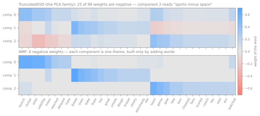
SVD's components contain 25 negative weights. Its component 2 reads "sports words, minus space words": a direction that separates two themes well, and a poor description of either. NMF can only build a document by adding parts, so each part ends up being one whole theme; this is the "parts-based" representation of Lee & Seung's paper, where NMF learned noses and eyes from face images while PCA learned signed "eigenfaces" (figure script).

Below, the same comparison is computed live in your browser. NMF starts from random positive weights: press step a few times and watch its rows turn into themes while its error falls toward the SVD's, then change \(k\).

The dashed line is the error of the truncated SVD, the smallest that any product of rank \(k\) can reach, and NMF stays slightly above it. That small price buys rows that are whole themes, never "sports minus space".

NMF on the posts

tv = TfidfVectorizer(**settings)
T = tv.fit_transform(docs)                                  # same vocabulary as X, TF-IDF weights
nmf = NMF(n_components=4, init='nndsvda', max_iter=500, random_state=0).fit(T)
print(*top_words(nmf.components_, vocab, 8), sep='\n')
nmf_label = nmf.transform(T).argmax(axis=1)
print(f"ARI with the forums: {adjusted_rand_score(y, nmf_label):.3f}")

graphics thanks files image program file know windows
god jesus people believe christ faith bible christians
game team hockey players play games season nhl
space nasa launch shuttle moon orbit lunar earth
ARI with the forums: 0.767

The four NMF topics are the four forums: graphics, religion, hockey, space, with none of the mixing LDA showed. Agreement with the forums rises from 0.456 to 0.767. That is one run on one corpus: the lab finds a corpus where the order is reversed. The next section scores both more carefully.

How many topics, and are they any good?

LDA and NMF need the number of topics \(k\) in advance. There are no labels to cross-validate against, so the choice needs a score computed from the documents alone. Two families of scores are common.

Perplexity asks how well the model predicts words it has not seen: fit LDA on 80% of the posts and measure how surprised it is by the other 20%. Lower is better. It is LDA's own likelihood, so it exists only for probabilistic models.

Coherence asks whether a topic's top words belong together. The most common measures are built on how often the words co-occur in documents (Röder, Both & Hinneburg, 2015, compare dozens of them against human judgments). The simplest to compute by hand is the normalized pointwise mutual information (NPMI) of two words:

where \(P(w)\) is the fraction of documents containing \(w\). It is 0 when the two words are independent, 1 when they always appear together and \(-1\) when they never do. By hand, for god and jesus in the posts:

B = CountVectorizer(stop_words='english', token_pattern=r'(?u)\b[a-zA-Z]{3,}\b',
                    binary=True).fit(docs)                 # reference: which post contains which word
Xb = B.transform(docs).tocsc()
col = B.vocabulary_
D = Xb.shape[0]

def n_docs(*ws):                                           # number of posts containing all the words
    hit = np.ones(D, dtype=bool)
    for w in ws:
        hit &= Xb[:, col[w]].toarray().ravel() > 0
    return int(hit.sum())

n_i, n_j, n_ij = n_docs('god'), n_docs('jesus'), n_docs('god', 'jesus')
p_i, p_j, p_ij = n_i / D, n_j / D, n_ij / D
print(D, n_i, n_j, n_ij)
print(f"PMI = {np.log(p_ij / (p_i * p_j)):.3f}   NPMI = {np.log(p_ij / (p_i * p_j)) / -np.log(p_ij):.3f}")

2155 304 159 101
PMI = 1.505   NPMI = 0.492

Of the 2,155 posts, 304 contain god, 159 contain jesus and 101 contain both. If the words were independent, both would appear in \(0.141 \times 0.074 = 1.04\%\) of the posts; they appear together in \(101/2155 = 4.69\%\), 4.5 times more. \(\log 4.5 = 1.505\), divided by \(-\log 0.0469 = 3.06\), gives an NPMI of 0.492. The coherence of a topic is the mean NPMI over all pairs of its top-10 words, and the coherence of a model is the mean over its topics. A second, simpler score, topic diversity (Dieng, Ruiz & Blei, 2020), is the fraction of distinct words among the top words of all topics: 1.0 when no two topics share a top word.

from itertools import combinations

def npmi(w1, w2):
    p1, p2, p12 = n_docs(w1) / D, n_docs(w2) / D, n_docs(w1, w2) / D
    return -1.0 if p12 == 0 else np.log(p12 / (p1 * p2)) / -np.log(p12)

def coherence(topics, n=10):           # mean NPMI over all pairs of each topic's top-n words
    return np.mean([np.mean([npmi(a, b) for a, b in combinations(t.split()[:n], 2)])
                    for t in topics])

def diversity(topics, n=10):           # share of distinct words among all topics' top-n words
    ws = [w for t in topics for w in t.split()[:n]]
    return len(set(ws)) / len(ws)

for name, comp in [('LDA', lda.components_), ('NMF', nmf.components_)]:
    tops = top_words(comp, vocab, 10)
    print(f"{name}  coherence (NPMI) {coherence(tops):.3f}   diversity {diversity(tops):.2f}")

LDA  coherence (NPMI) 0.224   diversity 0.85
NMF  coherence (NPMI) 0.369   diversity 1.00

Both scores agree with what we saw by eye: NMF's topics are more coherent (0.369 against 0.224) and share no top word, while LDA repeats words such as space, like and think across topics. Now the question of \(k\). The figure computes both scores for \(k\) from 2 to 20, with three seeds per point (figure script):

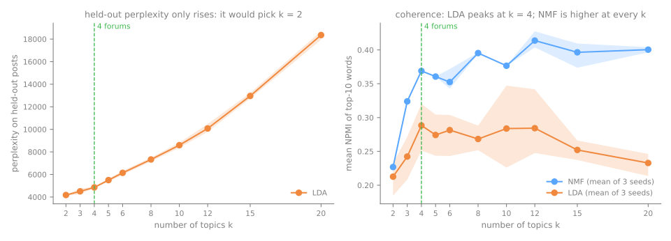
• Held-out perplexity only rises. Read literally, it recommends \(k = 2\). This behavior of scikit-learn's perplexity is well known, and a bigger problem is that even when perplexity behaves, it does not track what people find interpretable: Chang et al. (2009) found that models with better perplexity often had topics humans judged worse.
• Coherence peaks for LDA at \(k = 4\), the number of forums, though its seed-to-seed band is almost as wide as the whole curve. NMF's coherence jumps up to \(k = 4\) and then stays on a plateau: past that point, NMF splits the forums into sub-themes that are just as coherent.

The practical rule: scan a range of \(k\), look at the coherence curve for a knee rather than a maximum, and then read the topics at two or three candidate values. The number of topics is a choice about granularity (four forums, or twelve sub-themes?), and no score makes that choice for you.

References

• Lee, D. D.; Seung, H. S. "Learning the Parts of Objects by Non-negative Matrix Factorization." Nature 401 (1999): 788–791 — NMF and parts-based representations. DOI
• Röder, M.; Both, A.; Hinneburg, A. "Exploring the Space of Topic Coherence Measures." WSDM (2015): 399–408 — coherence measures compared with human judgments. DOI
• Chang, J.; Boyd-Graber, J.; Gerrish, S.; Wang, C.; Blei, D. M. "Reading Tea Leaves: How Humans Interpret Topic Models." NeurIPS 22 (2009) — better perplexity does not mean more interpretable topics.
• Dieng, A. B.; Ruiz, F. J. R.; Blei, D. M. "Topic Modeling in Embedding Spaces." TACL 8 (2020): 439–453 — where the topic diversity score comes from. DOI

Next: U5.3 BERTopic, topics as clusters of documents.