Cross-Validation and Data Leakage
In the last lessons every choice was made the same way. The k of k-nearest neighbors (k-NN), the decision threshold and the class_weight of the lesson on ROC (receiver operating characteristic) and PR (precision–recall) curves for imbalanced data: carve a validation set out of the training data, try the options on it and keep the best. This lesson shows that a single split is a lottery (the answer depends on which rows landed in it) and replaces it with cross-validation (CV). Then it turns the golden rule — never evaluate on training data — into engineering practice: how to spot data leakage, and how to compare models without fooling yourself.
Every claim below is measured, not just stated: each figure is produced by a short Python script next to this page, and the code blocks reproduce the numbers quoted in the text.
How this lesson is organized
The lesson has two approaches. Each one has slides, text and a lab to run in class on Colab; the quiz at the end covers the fundamental one. Start with the fundamental one: the advanced one builds on it.
| Fundamental approach | Advanced approach | |
|---|---|---|
| question | How do you measure a recipe's performance without depending on the luck of one split? | How not to fool yourself: leakage, unfair comparisons and the winner's curse |
| content | train/validation/test, why one split is a lottery, k-fold, CV schemes, preprocessing per fold | the five leakage patterns, paired comparison, the tie rule, nested CV, resampling inside the folds |
| in-class lab | breast cancer: CV in action, steps 1 to 6 | compare, check and test, steps 7 to 13 |
| by the end, you can | build train/validation/test; run k-fold and read mean ± std; pick the right CV scheme; tune a hyperparameter with a grid search | recognize the five leaks and measure them; compare candidates fold by fold; declare ties; know how much your own tuning inflates the number |
Both labs use the same notebook on Colab (in Portuguese): the fundamental part runs steps 1 to 6, the advanced part steps 7 to 13. Everything runs in the browser; there is nothing to download.
Fundamental approach
One question guides this part: how do you measure a recipe's performance without depending on the luck of one split? The answer is to trade one validation set for \(k\) of them and report mean ± standard deviation.
This part follows one pipeline in four stages, drawn below: 1. three sets, the roles of train, validation and test; 2. one split → k folds, cross-validation against the luck of one split; 3. honest folds, the right splitter and preprocessing refit in every fold; 4. the honest recipe, put to work in the lab. Each stage links to its section, and in the slides a strip at the bottom shows which stage you are in.
- Three setstrain, validation, test; why validation wears out
- One split → k foldsthe lottery of one split, k-fold, mean ± std
- Honest foldsthe right splitter, preprocessing refit in every fold
- The honest recipefive rules, then the lab: tune C with a grid search
Slides: fundamental approach
Click the slides and use the ← → arrows to navigate; F goes full screen and Esc shows every slide. Open the slides in a new tab
1. Train / validation / test
Stage 1. Before any model, decide which data may judge it: three sets, three roles.
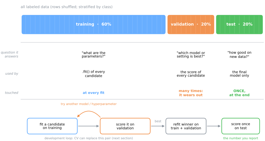
- Training set — the model learns its parameters here;
- Validation set — used to choose between models and hyperparameter values. Because you make decisions on it, performance on it becomes optimistically biased over time;
- Test set — simulates the future. Used once, at the very end. If you iterate against the test set, it silently becomes a validation set and you no longer have an honest estimate.
The bottom row is the workflow. The development loop — fit on training, score on validation, try something else — runs as many times as you like; that repetition is exactly what wears the validation set out. Once a winner is chosen, it is usually refit on training + validation (more data, same recipe), and only then does the test set speak, once (figure script). In code:
from sklearn.datasets import load_breast_cancer
from sklearn.model_selection import train_test_split

X, y = load_breast_cancer(return_X_y=True)                      # any table of features and labels
X_temp, X_test, y_temp, y_test = train_test_split(X, y, test_size=0.2, random_state=42,
                                                  stratify=y)   # keep class ratios
X_train, X_val, y_train, y_val = train_test_split(X_temp, y_temp, test_size=0.25,
                                                  random_state=42, stratify=y_temp)
print(len(X_train), len(X_val), len(X_test))
The result is a 60/20/20 split: test_size=0.25 of the remaining 80% is 20% of the whole. stratify=y preserves class proportions in every split — important for imbalanced classification (see ROC, PR & Imbalanced Data).
Why a set you choose on stops being honest
"Performance on the validation set becomes optimistically biased" sounds abstract. It is easiest to see where there is nothing to find. Take a dataset of pure noise — 20 random columns and a coin-flip target — so that no model can truly beat 50%. Split it 50/25/25, train 100 decision trees with random hyperparameters (the trees come in the decision trees lesson; any model with knobs would do), and do what everyone does: keep the one with the best validation score.
import numpy as np
from sklearn.model_selection import train_test_split
from sklearn.tree import DecisionTreeClassifier

rng = np.random.default_rng(0)
X, y = rng.normal(size=(400, 20)), rng.integers(0, 2, 400)       # no signal at all
X_tmp, X_te, y_tmp, y_te = train_test_split(X, y, test_size=0.25, random_state=0)
X_tr, X_va, y_tr, y_va = train_test_split(X_tmp, y_tmp, test_size=1/3, random_state=0)

results = []
for k in range(100):                                             # 100 "configurations"
    m = DecisionTreeClassifier(max_depth=int(rng.integers(1, 8)),
                               max_features=int(rng.integers(1, 21)),
                               random_state=k).fit(X_tr, y_tr)
    results.append((m.score(X_va, y_va), m.score(X_te, y_te)))

best_val, its_test = max(results, key=lambda r: r[0])           # pick on validation
print(f"winner on validation: {best_val:.1%}   same model on test: {its_test:.1%}")
Repeating the experiment 30 times and averaging gives the figure below (script):
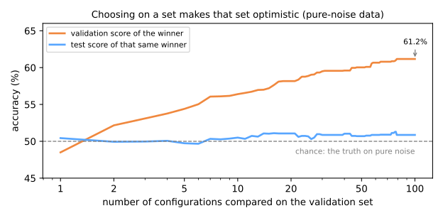
With one configuration, validation and test agree: both hover at 50%. As you compare more, the winner's validation score climbs to 61.2%, while the same winner, measured on untouched data, stays at 50.9%. No model got better. You simply picked whichever one happened to agree with the random quirks of those 100 validation rows; the more candidates, the bigger the lucky quirk you find. This is the winner's curse, and it is the entire reason for the rules above:
- the score of the selected model on the set used to select it is biased upward — by an amount that grows with the number of things you tried;
- a set that played no part in any decision is the only one whose score you can quote. That is the test set, and it stays honest only while you make no decision on it.
On real data the gap is smaller, because true signal dominates the lucky quirks, but on average it points the same way.
2. Cross-validation
A single split is a lottery
Stage 2. A single validation split has a second problem, independent of the first: its result depends on which rows happened to land in it. Keep everything fixed — the breast-cancer dataset (569 rows), a scaled logistic regression — and change only the random_state of an 80/20 split:
from sklearn.datasets import load_breast_cancer
from sklearn.linear_model import LogisticRegression
from sklearn.model_selection import StratifiedKFold, cross_val_score, train_test_split
from sklearn.pipeline import make_pipeline
from sklearn.preprocessing import StandardScaler

X, y = load_breast_cancer(return_X_y=True)
pipe = make_pipeline(StandardScaler(), LogisticRegression(max_iter=1000))

for seed in [0, 1, 2, 3, 4]:
    X_tr, X_va, y_tr, y_va = train_test_split(X, y, test_size=0.2, random_state=seed, stratify=y)
    print(seed, f"{pipe.fit(X_tr, y_tr).score(X_va, y_va):.3f}")
Doing this for 300 seeds (script):
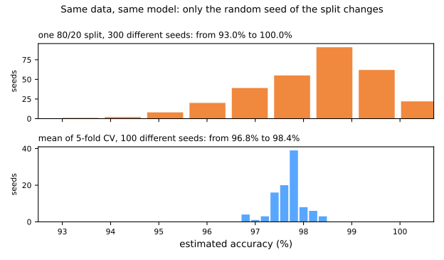
The same model, on the same data, "scores" anywhere from 93.0% to 100.0%, with a standard deviation of 1.3 points. A student who reports 100% and a student who reports 93% may have written identical code. With 114 validation rows, one row is worth 0.88 points of accuracy, so a handful of hard cases landing on one side or the other is enough to swing the result.
The bottom panel is the fix: the mean of a 5-fold cross-validation, over 100 different shuffles, stays between 96.8% and 98.4% (standard deviation 0.34 — four times smaller). Both estimates are centered on the same value; cross-validation is not more optimistic, only much less at the mercy of luck.
The simulator below runs the same experiment on a two-class dataset whose true accuracy we know (78%, measured on 20,000 fresh points). With \(n = 80\) rows (the slider n is the number of rows), press Draw 100: the hold-out lands anywhere between roughly 60% and 100%, while the CV mean stays inside a band a few points wide. Then press New dataset a few times.
The second experiment shows what cross-validation does not fix. With \(n = 80\), the narrow blue band sits at 80.0–87.5% for one dataset and at 72.5–78.8% for the next — sometimes away from the white line. CV greatly reduces the luck of the split; it cannot remove the luck of the sample, because every fold is drawn from the same 80 rows. A small dataset that happens to be easy looks easy under any validation scheme. Only more data helps: move the slider to 600 and the CV band shrinks to about 2 points, close to the truth, while a single hold-out still spans about 20. This is why a mean ± std from CV should be read as "how this recipe performs on data like mine", with the "like mine" carrying real weight when \(n\) is small.
k-fold, step by step
k-fold cross-validation (typically \(k = 5\) or \(10\)):
- partition the training data into \(k\) folds;
- for each fold: train on the other \(k-1\), evaluate on it;
- report the mean (and standard deviation!) of the \(k\) scores.
from sklearn.model_selection import cross_val_score, StratifiedKFold, train_test_split

X_train, X_test, y_train, y_test = train_test_split(X, y, test_size=0.2, random_state=42,
                                                    stratify=y)   # CV replaces the validation set
cv = StratifiedKFold(n_splits=5, shuffle=True, random_state=42)
scores = cross_val_score(pipe, X_train, y_train, cv=cv, scoring='f1')
print(scores.round(3))
print(f"{scores.mean():.3f} ± {scores.std():.3f}")
Every observation serves as validation exactly once, and the model is scored on all the rows instead of 20% of them — that is where the reduction in variance comes from. The price is \(k\) fits instead of one. The spread of the \(k\) scores is information too: if the folds read 0.97, 0.96, 0.98, 0.71, 0.97, the mean hides a model that fails badly on some subset of the data, and that fold deserves a look.
The \(k\) models are thrown away afterwards. CV evaluates a recipe (algorithm + hyperparameters + preprocessing); the model you ship is that recipe refit once on all the training data.
Choosing a CV scheme
Stage 3. The splitters differ only in which rows they are allowed to put together in a validation fold. The picture makes that concrete. Here are 60 rows as they often sit in a real file — sorted by class (the 12 positives at the end) and by patient (12 patients of different sizes, one block each in the purple strip) — and the five folds each splitter produces (script):
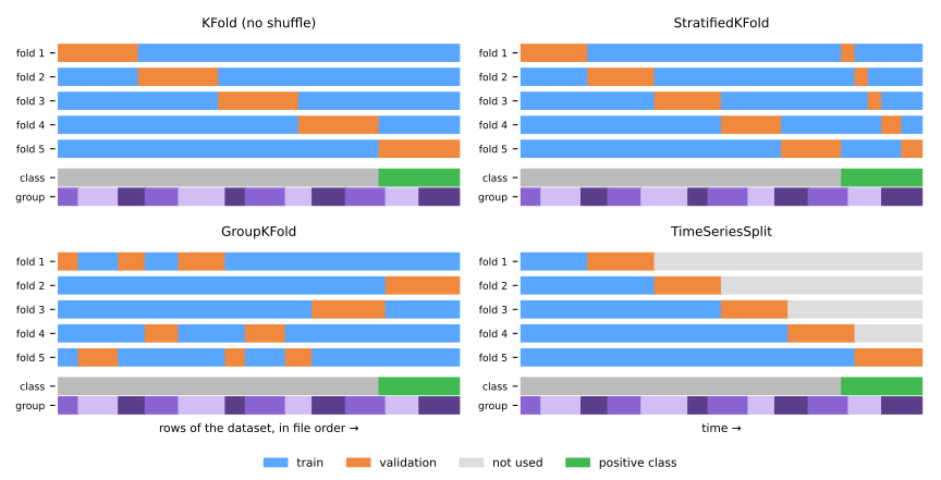
- KFold without shuffling cuts the file into consecutive blocks. Because the file is sorted, fold 5 validates on all positives, and folds 1–4 validate on none — four folds on which recall is undefined. Always pass
shuffle=Trueunless the order is meaningful (time); - StratifiedKFold takes the same fraction of each class into every fold: each validation fold gets 2–3 positives;
- GroupKFold never splits a patient: each purple block lands entirely in one validation fold, so the model is always scored on patients it has never seen;
- TimeSeriesSplit only ever validates on the future of its training window; the training window grows, and the gray part (the future of the future) is not used.
Shuffling is not enough to make KFold safe on imbalanced data. With 100 rows and 8 positives:
import numpy as np
from sklearn.model_selection import KFold, StratifiedKFold

y = np.array([1] * 8 + [0] * 92); X = np.zeros((100, 1))
for name, cv in [('KFold', KFold(5)),
                 ('KFold shuffled', KFold(5, shuffle=True, random_state=0)),
                 ('StratifiedKFold', StratifiedKFold(5, shuffle=True, random_state=0))]:
    print(f"{name:16s}", [int(y[va].sum()) for _, va in cv.split(X, y)])
Positives per validation fold. Across 1,000 seeds, the shuffled KFold left at least one fold with zero positives 65% of the time. Stratification guarantees 1 or 2 in every fold.
| Method | When to use | Advantages | Watch out for |
|---|---|---|---|
| K-Fold | regression, balanced data (with shuffle=True) | simple, efficient | folds can miss a rare class entirely |
| Stratified K-Fold | classification (especially imbalanced) | keeps class proportions in every fold | only stratifies on the target |
| Leave-One-Out (LOO) | very small datasets (< 100–200 samples) | uses almost all data for training | very slow (\(n\) fits, one per row); each fold scores a single row (right or wrong), so the per-fold std means nothing and recall or the area under the ROC curve (AUC) cannot be computed per fold: pool the predictions with cross_val_predict |
| TimeSeriesSplit | temporal data / time series | respects chronological order | early folds train on little data; add gap when the target looks ahead |
| Group K-Fold | grouped data (patients, users, ...) | prevents leakage between related rows | requires a group column |
scikit-learn's default when you write cv=5 is StratifiedKFold for classifiers and unshuffled KFold otherwise. The test set stays outside the whole procedure: cross-validation replaces the validation set, not the test set.
Preprocessing must restart in every fold
Scaling, encoding, imputation, and feature selection must be re-fit from scratch inside each fold. If you StandardScaler().fit_transform() or SelectKBest().fit() on the whole dataset before cross_val_score/GridSearchCV, the validation fold's statistics leak into training. For a step that looks at y (feature selection, target encoding) the score comes out optimistic, sometimes wildly; for one that does not (a scaler, a mean imputer) the error is usually small and can go either way (Moscovich & Rosset, 2022), but you only know its size by measuring. Passing a Pipeline makes this automatic: in every fold, all steps are fit only on that fold's training portion, then applied frozen to the validation portion. Each fold gets its own scaler, its own selected features, and its own model. How large the resulting error can be is measured in the advanced approach.
Key idea
Cross-validation scores a recipe, not a model: algorithm + hyperparameters + preprocessing. The \(k\) fitted models are thrown away; what goes to production is the same recipe refit once on all the training data.
3. Summary: the honest-validation recipe
Stage 4. Everything above, as a recipe to follow, then put to work in the lab:
- Lock the test set away before anything else, with
stratifyfor classification. - Replace the validation split with CV:
StratifiedKFold(5, shuffle=True, random_state=...)for classification. - Build every candidate as a
Pipeline, with every fitted step inside, so CV refits it in each fold. - Report mean ± std, never the mean alone, and look at the individual folds before trusting the mean.
- Reuse a single
cvobject across all candidates, so the comparison is paired.
| common mistake | symptom | fix |
|---|---|---|
KFold without shuffling on a sorted file | folds with no rows of one class | shuffle=True, or StratifiedKFold |
scaling or selecting before cross_val_score | a wrong score, with no warning; optimistic if the step looks at y | the step inside the Pipeline |
| quoting only the mean of the folds | "0.95" hides whether it is ± 0.005 or ± 0.05 | always mean ± std |
| iterating against the test set | it becomes a validation set | decide on CV, touch the test once |
Fundamental lab — CV in action
A complete experiment, from raw table to a single honest number, using everything above. The setting: a screening tool that flags breast tumours as malignant from 30 measurements of a biopsy image. A missed cancer is far worse than a false alarm, so the metric we care about is recall on the malignant class, with the area under the ROC curve (ROC AUC) alongside. Two families compete: the logistic regression, with its regularization strength C and its class_weight, and k-NN, with n_neighbors and weights. Steps 3 to 6 cross-validate the logistic regression and tune its C; steps 7 to 13 live in the advanced lab.
How to run this lab in class (about 35 min, in pairs)
- Open the lab notebook on Colab (in Portuguese). There is nothing to download or install: Colab runs in the browser. To keep your answers, save a copy to your Drive (File → Save a copy in Drive) before editing. Run the cells in order, in one session.
- This lab covers steps 1 to 6 of the notebook. The advanced lab continues in the same notebook, from step 7.
- Each step starts with a Predict: answer it with your partner before running the cell. Getting the prediction wrong is what makes the result stick.
- After running, compare with the output and the reading on this page. Every output here is exactly what the code prints.
- The Simulations ask you to write a small Python experiment: change one input and watch what happens to the output. No arithmetic by hand. The solution is collapsed right below: try before opening it.
- Suggested pace: steps 1 to 3 in 10 min; step 4 and its simulation in 12 min; steps 5 and 6 with the simulation in 13 min.
Step 1 — load and fix the label
Predict. In scikit-learn's copy, target = 1 is benign. If you computed "recall" without touching that, what exactly would you be measuring?
import numpy as np
import pandas as pd
from sklearn.datasets import load_breast_cancer

data = load_breast_cancer(as_frame=True)
X = data.data                     # 30 numeric measurements of each tumour
y = 1 - data.target               # scikit-learn codes benign = 1; flip so that 1 = malignant
print(X.shape)
print(y.value_counts())
Check what 1 means before computing anything. In scikit-learn's copy of this dataset, target = 1 is benign. Left as is, "recall" would measure how well we find healthy patients. We flip the label so that the positive class is the one we are trying to catch: 212 malignant (37%) against 357 benign.
Step 2 — lock the test set away
Predict. This is the only split made by hand in the whole lab. Why does stratify matter here, with 37% malignant? Until which step must X_test stay untouched?
from sklearn.model_selection import train_test_split

X_train, X_test, y_train, y_test = train_test_split(
    X, y, test_size=0.2, stratify=y, random_state=42)
print(X_train.shape, X_test.shape)
print(f"malignant share: train {y_train.mean():.3f} · test {y_test.mean():.3f}")
This is the only split we make by hand. From here until step 12, X_test and y_test are not touched. stratify=y keeps the 37% malignant share identical on both sides.
Step 3 — a baseline, so the numbers mean something
Predict. What accuracy will a model that always answers "benign" reach, with 37% malignant? And what recall?
from sklearn.dummy import DummyClassifier
from sklearn.model_selection import StratifiedKFold, cross_val_score

cv = StratifiedKFold(n_splits=5, shuffle=True, random_state=42)

dummy = DummyClassifier(strategy='most_frequent')          # always says "benign"
for metric in ['accuracy', 'recall']:
    s = cross_val_score(dummy, X_train, y_train, cv=cv, scoring=metric)
    print(f"{metric:8s} {s.mean():.3f}")
A model that always answers "benign" gets 62.6% accuracy and catches zero cancers. Any accuracy below that is worse than doing nothing, and even 90% is not very impressive on this data. This is why the rest of the lab tracks recall. The cv object defined here is reused in every later step, so every comparison uses the same five folds.
Step 4 — 5-fold CV with several metrics
Predict. Will the five folds give the same recall? If they differ, would you say the difference comes from the model or from which tumours landed in each fold?
from sklearn.linear_model import LogisticRegression
from sklearn.model_selection import cross_validate
from sklearn.pipeline import make_pipeline
from sklearn.preprocessing import StandardScaler

model = make_pipeline(StandardScaler(), LogisticRegression(max_iter=1000))

res = cross_validate(model, X_train, y_train, cv=cv, return_train_score=True,
                     scoring=['accuracy', 'precision', 'recall', 'f1', 'roc_auc'])
folds = pd.DataFrame(res).drop(columns=['fit_time', 'score_time'])
print(folds[['train_recall', 'test_accuracy', 'test_precision', 'test_recall', 'test_roc_auc']].round(3))
print(folds.agg(['mean', 'std']).T.round(3))
   train_recall  test_accuracy  test_precision  test_recall  test_roc_auc
0         0.978          0.956           1.000        0.882         0.995
1         0.963          0.967           0.943        0.971         0.999
2         0.963          1.000           1.000        1.000         1.000
3         0.978          0.978           1.000        0.941         0.987
4         0.971          0.967           0.943        0.971         0.998
                  mean    std
test_accuracy    0.974  0.017
train_accuracy   0.988  0.004
test_precision   0.977  0.031
train_precision  0.997  0.004
test_recall      0.953  0.045
train_recall     0.971  0.007
test_f1          0.964  0.023
train_f1         0.984  0.005
test_roc_auc     0.996  0.005
train_roc_auc    0.998  0.001
How to read it:
- Fold by fold. Recall ranges from 0.882 in fold 0 to 1.000 in fold 2. Each validation fold holds 34 malignant tumours, so 0.882 means 4 missed and 1.000 means none. Same model, same data: the difference is which tumours landed in which fold, the "luck of the split" measured at the start of this lesson.
- Mean ± std. The honest summary is recall 0.953 ± 0.045 and ROC AUC 0.996 ± 0.005. Quote the std along with the mean: a recall of 0.95 ± 0.05 and one of 0.95 ± 0.005 are very different claims.
- Train vs validation. Training recall is 0.971 and validation recall 0.953, a gap of under 2 points. (The std printed here, 0.045, comes from
pandas, which divides by \(k-1\); thenumpyof steps 6 and 8 gives 0.040 on the same five folds.) The model is not overfitting much. It is not underfitting either: both numbers are high. - No leakage. The scaler sits inside the pipeline, so
cross_validaterefits it on each fold's 364 training rows.
Simulation: the luck of the split, measured. The lesson claimed a single split is a lottery. Measure it on the lab's own data: over 20 seeds, compare the accuracy of one 80/20 hold-out with the mean of a 5-fold CV. What range does each one cover?
Solution
single, kfold = [], []
for seed in range(20):
    Xa, Xb, ya, yb = train_test_split(X_train, y_train, test_size=0.2, stratify=y_train,
                                      random_state=seed)
    single.append(model.fit(Xa, ya).score(Xb, yb))        # a single hold-out
    k = StratifiedKFold(5, shuffle=True, random_state=seed)
    kfold.append(cross_val_score(model, X_train, y_train, cv=k, scoring='accuracy').mean())
for name, v in [('one 80/20 hold-out', single), ('5-fold CV mean', kfold)]:
    v = np.array(v)
    print(f"{name:20s} from {v.min():.3f} to {v.max():.3f}   std {v.std():.3f}")
Same model, same data, 20 different reports. With one hold-out the grade runs from 93.4% to 100.0%: two pairs with identical code can report numbers almost 7 points apart, and the luckier one looks like it did better work. The CV mean spans less than a point and a half (five times smaller spread), because each seed only reshuffles which rows land in which fold — all of them get validated anyway. That is why CV, not a split, is what you report.
Step 5 — a steadier mean: repeated CV
Predict. Repeating the 5-fold CV ten times with different shuffles — does it change the mean more, or your confidence in it?
from sklearn.model_selection import RepeatedStratifiedKFold

rcv = RepeatedStratifiedKFold(n_splits=5, n_repeats=10, random_state=42)
rec = cross_val_score(model, X_train, y_train, cv=rcv, scoring='recall')
print(f"{len(rec)} scores · recall {rec.mean():.3f} ± {rec.std():.3f} · "
      f"from {rec.min():.3f} to {rec.max():.3f}")
The recall from step 4 depends on how those particular five folds happened to be cut. Repeating 5-fold CV ten times with different shuffles gives 50 scores and a mean (0.947) that depends much less on one choice of random_state. The spread of individual folds, 0.853 to 1.000, is a useful reminder of how noisy a single fold with 34 positives is. The price is 50 fits instead of 5, which is trivial here.
Step 6 — tune C with a grid search
Predict. Small C means strong penalty. At C = 0.001, will training and validation recall both be low, both high, or far apart? And at C = 1000?
Recall that C plays the role of \(1/\alpha\), the inverse of the penalty strength \(\alpha\) of Ridge (up to a constant factor): small C = strong penalty.
from sklearn.model_selection import GridSearchCV

grid = GridSearchCV(model, {'logisticregression__C': np.logspace(-3, 3, 13)},
                    cv=cv, scoring='recall', return_train_score=True)
grid.fit(X_train, y_train)

table = pd.DataFrame(grid.cv_results_)[['param_logisticregression__C', 'mean_train_score',
                                        'mean_test_score', 'std_test_score']]
table.columns = ['C', 'train recall', 'val recall', 'val std']
print(table.round(3).to_string(index=False))
print(f"best: C = {grid.best_params_['logisticregression__C']:g} · recall {grid.best_score_:.3f}")
       C  train recall  val recall  val std
   0.001         0.694       0.700    0.088
   0.003         0.843       0.841    0.084
   0.010         0.878       0.865    0.061
   0.032         0.929       0.912    0.042
   0.100         0.957       0.935    0.043
   0.316         0.965       0.947    0.051
   1.000         0.971       0.953    0.040
   3.162         0.978       0.941    0.037
  10.000         0.978       0.941    0.032
  31.623         0.985       0.941    0.032
 100.000         0.997       0.947    0.022
 316.228         1.000       0.947    0.022
1000.000         1.000       0.947    0.022
best: C = 1 · recall 0.953
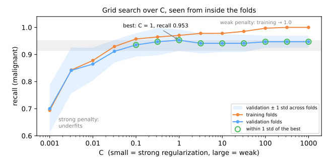
The figure shows the table. Small C means strong regularization: at C = 0.001 the coefficients are crushed toward zero and the model misses 30% of cancers on training and validation. That is underfitting, visible because the two curves sit together at a low value. Toward large C, training recall climbs to 1.000 while validation stays around 0.94–0.95, so the gap opens: the beginning of overfitting.
The grid search picks C = 1 with 0.953. Look at the green circles before celebrating: every C from 0.1 to 1000 is within one fold-standard-deviation (0.040) of the winner. That yardstick is rough: all thirteen values were scored on the same five folds, and comparing them fold by fold is sharper (the solution of the simulation below does it). Here both agree: the differences are no larger than the noise between folds, so the evidence does not show that C = 1 beats the others. Picking C = 1 is fine. Claiming that C = 1 is better than C = 10 is not. It is also the winner's curse again: 0.953 is the best of 13 noisy estimates, so it is slightly optimistic.
So far only one family has been tuned, and only one of its knobs. Steps 7 to 9, in the advanced lab, widen the search and put a second family next to it.
Simulation: the one-standard-error rule. The search picked C = 1, but the figure suggests a plateau. Apply the one-standard-error rule (Breiman et al., 1984): compute the standard error of the best mean (the between-fold std divided by \(\sqrt{5}\)), see how many configurations fall inside it, and keep the simplest — here, the most regularized C.
Solution
t = pd.DataFrame(grid.cv_results_)[['param_logisticregression__C', 'mean_test_score', 'std_test_score']]
t.columns = ['C', 'recall', 'std']
i = t['recall'].idxmax()
se = t.loc[i, 'std'] / np.sqrt(5)                          # standard error of the best mean
ok = t[t['recall'] >= t.loc[i, 'recall'] - se]
print(f"best: C = {t.loc[i, 'C']:g}, recall {t.loc[i, 'recall']:.3f}, one standard error = {se:.3f}")
print(f"within one SE: C from {ok['C'].min():g} to {ok['C'].max():g} ({len(ok)} of {len(t)} configurations)")
print(f"simplest (most regularized) C in that range: C = {ok['C'].min():g}, recall {ok.loc[ok['C'].idxmin(), 'recall']:.3f}")

folds = np.array([grid.cv_results_[f'split{k}_test_score'] for k in range(5)]).T   # 13 C values x 5 folds
d = folds[i] - folds                                       # C = 1 minus each C, fold by fold
tie = d.mean(axis=1) < d.std(axis=1)                       # paired rule: mean difference within its spread
print(f"paired ties with C = 1: C from {t['C'][tie].min():g} to {t['C'][tie].max():g}")
for j in [3, 4, 8]:                                        # C = 0.0316, 0.1 and 10
    print(f"C = 1 minus C = {t.loc[j, 'C']:<6.3g} in tumours per fold: {np.round(d[j] * 34).astype(int)}")
best: C = 1, recall 0.953, one standard error = 0.018
within one SE: C from 0.1 to 1000 (9 of 13 configurations)
simplest (most regularized) C in that range: C = 0.1, recall 0.935
paired ties with C = 1: C from 0.1 to 1000
C = 1 minus C = 0.0316 in tumours per fold: [1 0 3 2 1]
C = 1 minus C = 0.1    in tumours per fold: [1 0 2 0 0]
C = 1 minus C = 10     in tumours per fold: [0 0 2 0 0]
Nine of the thirteen configurations fall within one standard error of the winner. The one-standard-error rule picks the simplest among them: C = 0.1, ten times more regularized than C = 1, for a loss of 0.018 in recall that the one-standard-error convention treats as noise. The last lines repeat the comparison fold by fold, the sharper paired check of the advanced part (each fold holds 34 malignant tumours): every C from 0.1 to 1000 is a tie with C = 1 by that rule too. Against C = 0.1 and C = 10, C = 1 catches at most two more tumours in a fold and the same number in most folds; against C = 0.0316 it catches more in four folds of five, and that is not a tie. Choosing C = 1 is still defensible; what is not defensible is claiming that C = 1 beats C = 10. The rule is a convention for not paying for complexity the data cannot confirm.
To close the fundamental part. One sentence each: (1) what does cross-validation score, a model or a recipe? (2) Why must the between-fold std be reported next to the mean? (3) What happens if StandardScaler is fit before cross_val_score?
Your turn (fundamental)
For homework:
- How many folds? Repeat step 4 with
cv=StratifiedKFold(3, ...)and with10. What happens to the mean and to the between-fold std? What does it cost in fitting time? - Without stratifying. Replace the
StratifiedKFoldof step 3 withKFold(5, shuffle=True, random_state=42)and look at how many malignant cases land in each validation fold (for _, va in cv.split(X_train, y_train): print(y_train.iloc[va].sum())). With 37% positives the difference is small; redo it imagining 3% and explain why stratifying would become mandatory. - Outside the pipeline. Fit a
StandardScaleron all ofX_train, transform, and runcross_val_scorewith theLogisticRegressionalone. Compare with step 4. Is the difference large here? Why can you not conclude from that that scaling outside the pipeline is safe?
Advanced approach
The fundamental part gave a stable estimate. This part asks how it can lie: information leaking into training, comparisons that measure who tried harder rather than which algorithm fits, and the winner's number, which is optimistic by construction. The code blocks in this part are independent: each one builds its own data.
This part follows one pipeline in four stages: 1. find the leaks, five patterns, each one measured; 2. compare fairly, metric first, tuned candidates on the same folds; 3. grade the winner, nested cross-validation and resampling inside the folds; 4. end to end, one leak-free experiment and the lab. Each stage links to its section, and in the slides a strip at the bottom shows which stage you are in.
- Find the leaksfive patterns, each one measured; the smell test
- Compare fairlymetric first, tuned candidates, same folds, ties
- Grade the winnernested cross-validation (CV), resampling inside the folds
- End to endthe steps in order, then the lab: compare, check and test
Slides: advanced approach
Click the slides and use the ← → arrows to navigate; F goes full screen and Esc shows every slide. Open the slides in a new tab
4. Data leakage
Stage 1. Leakage = information from outside the training fold sneaking into training. The model looks brilliant in evaluation and collapses in production, where the leaked information does not exist yet.
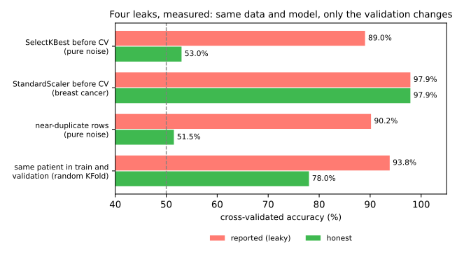
The figure below summarizes four of the classic patterns, each measured twice on the same data with the same model: once with the leak, once with an honest validation (script). The sections that follow take them one at a time.
1. Preprocessing before splitting
Fitting a scaler, imputer, or feature selector on all data before the split leaks test-set statistics into training. You met this in Preprocessing; the cure is structural — put every fitted step inside a Pipeline so it is re-fit within each fold.
How much it costs depends on what the step learns. Compare two steps, both fit before CV:
import numpy as np
from sklearn.feature_selection import SelectKBest, f_classif
from sklearn.linear_model import LogisticRegression
from sklearn.model_selection import StratifiedKFold, cross_val_score
from sklearn.pipeline import make_pipeline

rng = np.random.default_rng(5)
X, y = rng.normal(size=(100, 5000)), rng.integers(0, 2, 100)     # 5000 noise columns
cv = StratifiedKFold(n_splits=5, shuffle=True, random_state=0)

# WRONG: the selector looks at all 100 labels, then CV runs on the survivors
X_sel = SelectKBest(f_classif, k=20).fit_transform(X, y)
print(cross_val_score(LogisticRegression(max_iter=1000), X_sel, y, cv=cv).mean())   # 0.89

# RIGHT: the selector is re-fit inside each fold, on that fold's 80 training rows
pipe = make_pipeline(SelectKBest(f_classif, k=20), LogisticRegression(max_iter=1000))
print(cross_val_score(pipe, X, y, cv=cv).mean())                                    # 0.53
89% on data with no signal. Out of 5,000 random columns, some correlate with the labels by pure chance — including the labels of the rows that will later be used for validation. The selector picks exactly those, and every fold then "confirms" a pattern it helped choose. Inside the pipeline, the selector can only see the fold's training rows; its picks are then noise to the validation rows, and the score falls back to chance. This is not a toy: Ambroise & McLachlan (2002) found it in published gene-expression papers, where thousands of genes and a few dozen patients are the normal setting.
The same mistake with a StandardScaler on breast cancer changes nothing measurable here (97.9% both ways). A scaler learns only the mean and standard deviation of each column, never looks at y, and 569 rows pin those statistics down well. That is not a license: an imputer, a target encoder, an oversampler such as SMOTE (Synthetic Minority Over-sampling Technique) or anything else that looks at y or at a few rows can leak a lot, and you cannot know the size of the leak without running both versions (SMOTE is measured further down). The pipeline makes the question disappear.
Leakage, measured on pure noise
The simulator isolates the mechanism. Generate a coin-flip target and hundreds of columns of pure Gaussian noise. Nothing is learnable — an honest pipeline must land at 50%. Now select the single feature most correlated with the target, then split, then fit. The selection saw the test rows, and that is enough:
| noise columns | reported | honest |
|---|---|---|
| 20 | 58.9% | 50.4% |
| 120 | 63.0% | 50.7% |
| 300 | 65.8% | 49.9% |
The table is what the simulator displays with its default 60 samples; each value is the average of 200 draws. The honest bar refuses to move off chance, exactly as it should. The reported bar climbs with the number of columns, because with more columns there is a better chance that one of them correlates with the target by luck — and the selection step happily finds it. Sixteen points of accuracy, manufactured from nothing, by reordering two lines of code. It is the winner's curse from the first section again, this time hidden inside a preprocessing step.
2. Features that know the future
A column recorded after the prediction moment: predicting hospital readmission using number_of_followup_visits; predicting churn using account_closed_date is null. Flawless in the historical table, nonexistent at prediction time. No choice of CV scheme catches this one — the leak is in the columns, not the split. Ask of every feature: "is this value available at the moment the prediction must be made?"
3. Duplicate or near-duplicate rows
The same record (or trivially perturbed copies) landing in both train and test — common after data augmentation, oversampling, or joins. The model is graded on questions it memorized. To measure it, take 300 rows of noise with random labels and give every row a near-identical twin:
import numpy as np
from sklearn.model_selection import GroupKFold, KFold, cross_val_score
from sklearn.neighbors import KNeighborsClassifier

rng = np.random.default_rng(4)
X, y = rng.normal(size=(300, 10)), rng.integers(0, 2, 300)       # labels are coin flips
X2 = np.vstack([X, X + rng.normal(0, 0.01, X.shape)])             # each row + its twin
y2 = np.concatenate([y, y])
twin = np.concatenate([np.arange(300), np.arange(300)])           # which pair a row belongs to

knn = KNeighborsClassifier(n_neighbors=1)
print(cross_val_score(knn, X, y, cv=KFold(5, shuffle=True, random_state=0)).mean())    # 0.487
print(cross_val_score(knn, X2, y2, cv=KFold(5, shuffle=True, random_state=0)).mean())  # 0.902
print(cross_val_score(knn, X2, y2, cv=GroupKFold(5), groups=twin).mean())              # 0.515
The 90% is predictable by hand. A validation row's twin lands in the training folds with probability 4/5; then 1-NN (k-NN with a single neighbor) finds it and copies its label — always right. Otherwise it guesses — right half the time: \(0.8 \times 1 + 0.2 \times 0.5 = 0.9\). Remove duplicates before splitting, or, when copies are legitimate (several augmented versions of one image), keep each family in one fold with GroupKFold, as the last line does.
4. Group leakage
Multiple rows per entity (several images per patient, several orders per customer) split randomly: the model recognizes the patient, not the disease. The simulation: 60 patients, 10 exams each. Each patient has a strong personal "fingerprint" across 10 measurements (anatomy, the scanner used), and one measurement carries a weaker real sign of disease. The model is a random forest (the random forest lesson), used here as a black box.
import numpy as np
from sklearn.ensemble import RandomForestClassifier
from sklearn.model_selection import GroupKFold, KFold, cross_val_score

def patients(n_pat, seed, per=10):
    r = np.random.default_rng(seed)
    sick = r.integers(0, 2, n_pat)
    fingerprint = r.normal(0, 3, (n_pat, 10))
    pid = np.repeat(np.arange(n_pat), per)                       # patient id of each exam
    X = fingerprint[pid] + r.normal(0, 0.5, (n_pat * per, 10))
    X[:, 0] = 2.0 * sick[pid] + r.normal(0, 1, n_pat * per)      # the real signal
    return X, sick[pid], pid

X, y, pid = patients(60, seed=1)
rf = RandomForestClassifier(n_estimators=200, random_state=0)
print(cross_val_score(rf, X, y, cv=KFold(5, shuffle=True, random_state=0)).mean())  # 0.938
print(cross_val_score(rf, X, y, cv=GroupKFold(5), groups=pid).mean())               # 0.780

X_new, y_new, _ = patients(200, seed=99)                          # a new hospital
print(rf.fit(X, y).score(X_new, y_new))                                              # 0.7545
Random KFold reports 93.8%. With 10 exams per patient, about 7 of the other 9 sit in the training folds whenever one is validated, and the forest only needs to recognize the fingerprint to recall that patient's label. GroupKFold keeps every patient's exams in a single fold and reports 78.0%. The last line is the referee: 200 patients never seen before score 75.45% — the grouped estimate was the honest one. Always ask what is the unit I will predict on in production (a new patient, a new customer, a new store), and make that the unit of the split.
5. Temporal leakage
Random shuffling of time-stamped data trains the model on the future to predict the past. The starkest demonstration uses a series that cannot be predicted by construction: a random walk, where each day is the previous day plus a random Gaussian step. The only feature is the day number \(t\):
import numpy as np
from sklearn.ensemble import RandomForestRegressor
from sklearn.metrics import r2_score
from sklearn.model_selection import KFold, TimeSeriesSplit, cross_val_score

rng = np.random.default_rng(3)
t = np.arange(500).reshape(-1, 1)
price = 50 + np.cumsum(rng.normal(0, 1, 500))                     # a random walk

rf = RandomForestRegressor(n_estimators=200, random_state=0)
print(cross_val_score(rf, t, price, cv=KFold(5, shuffle=True, random_state=0)).mean())  #  0.99
print(cross_val_score(rf, t, price, cv=TimeSeriesSplit(5)).mean())                      # -1.78

naive = [r2_score(price[va], np.full(len(va), price[tr[-1]]))      # "tomorrow = last value seen"
         for tr, va in TimeSeriesSplit(5).split(t)]
print(np.mean(naive))                                                                   # -1.70
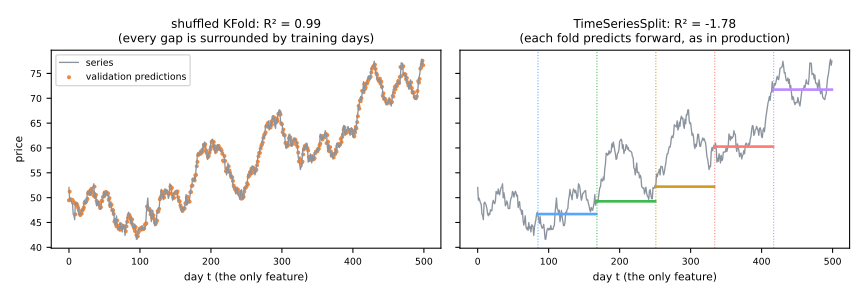
Shuffled KFold reports R² = 0.99 (R² is the coefficient of determination, 1 for a perfect fit; mean absolute error 0.67). On the left you can see why: every validation day is surrounded by training days, so the forest just reads off yesterday's and tomorrow's value. That is interpolation, and production never offers it — tomorrow's price is not in the table. TimeSeriesSplit asks the real question, predict days you have not reached yet, and the forest can only extend the last value it saw as a flat line: R² = −1.78 (mean absolute error 4.64). Do not read the negative sign as "worse than any sensible forecast": each fold's R² is measured against the mean of that validation fold, a value nobody knows in advance. The best honest forecast of a random walk, "tomorrow equals the last value seen", scores −1.70 on the same folds (the last line of the code). Here that is the correct answer: a random walk has nothing to learn. Always split chronologically, validate with TimeSeriesSplit, and build features only from values available before the moment being predicted (lags, rolling means that end yesterday).
The smell test
If results look too good — 99% accuracy on a hard problem, a feature with implausible importance, a huge gap between offline and production metrics — suspect leakage first, not genius. Check the top features in an explainability report: leaked features usually dominate it. And run the cheapest test there is: shuffle y at the very start and rerun the whole pipeline, preprocessing included. With random labels the score must fall to the shuffled baseline (chance for that model and metric, not necessarily 50%); if it does not, some step is learning from the labels outside the folds, like the selector of pattern 1. Passing proves less: duplicates, groups, time order and leaked columns lose their link to the shuffled labels too, so patterns 2 to 5 pass this test anyway.
5. Comparing models with cross-validation
Stage 2. The classification lessons left you with a shelf of candidates: a logistic regression, a k-NN with its k, and the remedies for imbalance, class_weight and resampling. So far each hyperparameter was chosen on a single validation split, and nothing told you which of them to ship. Cross-validation can answer that, as long as the comparison itself is fair. Six rules, each measured below:
- choose the metric from the problem, before looking at any model;
- tune every candidate before comparing them;
- score every candidate on the same folds, and compare them fold by fold;
- when two candidates are within the noise of each other, prefer the simpler one;
- the winner's score is optimistic: grade the whole choice with nested CV, or with the locked test set;
- resampling, like every other fitted step, happens inside the folds.
Choose the metric first
The data set is one of those on which SMOTE was introduced (Chawla et al., 2002), already met in the lab of the ROC and imbalanced data lesson: mammography, 11,183 small regions of mammograms, each described by 6 numbers computed from the image. Only 260 of them (2.3%) are calcifications, the finding a screening system must not miss. We lock a test set away first, then put five candidates through the same cv object:
import numpy as np
import pandas as pd
from sklearn.datasets import fetch_openml
from sklearn.dummy import DummyClassifier
from sklearn.linear_model import LogisticRegression
from sklearn.model_selection import StratifiedKFold, cross_validate, train_test_split
from sklearn.neighbors import KNeighborsClassifier
from sklearn.pipeline import make_pipeline
from sklearn.preprocessing import PolynomialFeatures, StandardScaler

mammo = fetch_openml(data_id=310, as_frame=True)
X, y = mammo.data, (mammo.target == '1').astype(int)            # 1 = calcification
X_dev, X_test, y_dev, y_test = train_test_split(X, y, test_size=0.2, stratify=y, random_state=0)
print(X_dev.shape, f"positives: {y_dev.sum()} ({y_dev.mean():.1%})")

cv = StratifiedKFold(n_splits=5, shuffle=True, random_state=0)  # ONE cv object for every candidate
candidates = {
    'dummy':             DummyClassifier(strategy='most_frequent'),
    'logistic':          make_pipeline(StandardScaler(), LogisticRegression(max_iter=1000)),
    'logistic balanced': make_pipeline(StandardScaler(),
                                       LogisticRegression(max_iter=1000, class_weight='balanced')),
    'logistic degree 2': make_pipeline(PolynomialFeatures(2), StandardScaler(),
                                       LogisticRegression(max_iter=1000)),
    'k-NN':              make_pipeline(StandardScaler(), KNeighborsClassifier()),
}
metrics = ['accuracy', 'roc_auc', 'average_precision']
results, rows = {}, {}
for name, est in candidates.items():
    results[name] = cross_validate(est, X_dev, y_dev, cv=cv, scoring=metrics)
    rows[name] = {m: f"{results[name]['test_' + m].mean():.3f} ± {results[name]['test_' + m].std():.3f}"
                  for m in metrics}
print(pd.DataFrame(rows).T)
(8946, 6) positives: 208 (2.3%)
                        accuracy        roc_auc average_precision
dummy              0.977 ± 0.000  0.500 ± 0.000     0.023 ± 0.000
logistic           0.983 ± 0.001  0.923 ± 0.036     0.622 ± 0.050
logistic balanced  0.901 ± 0.009  0.921 ± 0.034     0.585 ± 0.048
logistic degree 2  0.986 ± 0.001  0.948 ± 0.025     0.710 ± 0.043
k-NN               0.986 ± 0.002  0.904 ± 0.035     0.623 ± 0.070
Accuracy cannot tell the candidates apart: the dummy that never flags anything already scores 97.7%. ROC AUC squeezes the four real models between 0.90 and 0.95. With 2.3% positives, what matters is how clean the top of the ranking is, because the radiologist looks at the flagged regions first. That is average precision (AP, the area under the precision–recall curve of the ROC and imbalanced data lesson), and it separates the candidates: from 0.023 for the dummy (the prevalence, which is what a random ranking gets) to 0.710. It is the metric for the rest of this section. The metric is chosen from the problem, before looking at which model it favors; see Classification Metrics for the threshold metrics and the ROC and imbalanced data lesson for the ranking ones. The threshold itself is chosen later, for the winner only.
One row deserves a second look. class_weight='balanced' does not merely move the threshold: it changes the fitted coefficients, and here it makes the ranking worse (AP 0.585 against 0.622) while ROC AUC hardly moves. Class weights are a hyperparameter like any other, to be settled by cross-validation.
Tune every candidate before comparing
The table above compares models with their default settings. That measures the defaults, not the algorithms. Each family gets its own grid search, all on the same cv. The logistic regression's knob is C: by default scikit-learn's LogisticRegression adds to the cross-entropy the L2 penalty you met in Ridge, and C plays the role of \(1/\alpha\), the inverse of its strength (up to a constant factor): small C = strong penalty, large C = weak penalty, C=np.inf = the plain model of the logistic regression lesson.
from sklearn.model_selection import GridSearchCV

grids = {
    'logistic':          {'logisticregression__C': np.logspace(-3, 3, 7),
                          'logisticregression__class_weight': [None, 'balanced']},
    'logistic degree 2': {'logisticregression__C': np.logspace(-3, 3, 7)},
    'k-NN':              {'kneighborsclassifier__n_neighbors': [5, 15, 25, 35, 51, 75, 101],
                          'kneighborsclassifier__weights': ['uniform', 'distance']},
}
searches = {}
for name, grid in grids.items():
    searches[name] = GridSearchCV(candidates[name], grid, cv=cv, scoring='average_precision')
    searches[name].fit(X_dev, y_dev)
    s = searches[name]
    params = ', '.join(f"{k.split('__')[1]}={v}" for k, v in s.best_params_.items())
    print(f"{name:18s} {len(s.cv_results_['params']):2d} configs · "
          f"AP {s.best_score_:.3f} ± {s.cv_results_['std_test_score'][s.best_index_]:.3f} · {params}")
logistic           14 configs · AP 0.623 ± 0.050 · C=1000.0, class_weight=None
logistic degree 2   7 configs · AP 0.711 ± 0.049 · C=0.1
k-NN               14 configs · AP 0.712 ± 0.054 · n_neighbors=25, weights=distance
With defaults, the degree-2 logistic regression beat k-NN by 0.087 (0.710 against 0.623). Tuned, the gap is gone: 0.712 against 0.711. The default k = 5 was simply a bad setting for this problem. With 2.3% positives, most neighborhoods of 5 contain no calcification at all, and the score of a uniform k-NN (the fraction of positive neighbors) can take only 6 values, a very coarse ranking. With 25 neighbors weighted by distance the scores become fine-grained, and AP jumps. Had you tuned the logistic regressions and left k-NN at its default, you would have declared a winner that the data does not support. A tuned model against an untuned one measures who spent more effort, not which algorithm fits the problem.
The logistic grid also tried class_weight='balanced' and rejected it, confirming what the first table suggested.
Compare fold by fold
Every candidate has now been scored on the same five validation folds, so the scores come in pairs: fold 3 is the same 1,789 rows for every model. Look at the differences fold by fold, for two pairs: logistic against logistic balanced, and the two tuned leaders.
def fold_scores(search):
    """The 5 validation scores of the configuration GridSearchCV chose."""
    i = search.best_index_
    return np.array([search.cv_results_[f'split{k}_test_score'][i] for k in range(5)])

pairs = {'logistic - balanced': (results['logistic']['test_average_precision'],
                                 results['logistic balanced']['test_average_precision']),
         'k-NN - degree 2':     (fold_scores(searches['k-NN']),
                                 fold_scores(searches['logistic degree 2']))}
for name, (a, b) in pairs.items():
    d = a - b
    print(f"{name:20s} {a.round(3)} - {b.round(3)}")
    print(f"{'':20s} = {d.round(3)}  ->  {d.mean():+.3f} ± {d.std():.3f}")
logistic - balanced  [0.67  0.643 0.567 0.556 0.672] - [0.652 0.603 0.527 0.533 0.611]
                     = [0.018 0.04  0.041 0.023 0.061]  ->  +0.036 ± 0.015
k-NN - degree 2      [0.715 0.771 0.734 0.609 0.729] - [0.738 0.761 0.678 0.631 0.747]
                     = [-0.023  0.011  0.056 -0.022 -0.018]  ->  +0.001 ± 0.030
The first pair looks like a tie if you only read mean ± std: 0.622 ± 0.050 against 0.585 ± 0.048, two intervals that overlap almost completely. Fold by fold it is not a tie at all. The plain logistic wins every fold, by 0.036 ± 0.015. The large standard deviations come from the folds, not from the models: some folds are hard for everyone (fold 3 gives 0.556 and 0.533), others easy for everyone, and subtracting fold by fold cancels that shared difficulty. The second pair is a genuine tie: the mean difference, +0.001, is tiny next to its spread, 0.030, and the sign flips from fold to fold.
Five folds is not many. Repeating the 5-fold CV ten times with different shuffles gives 50 pairs:
from sklearn.model_selection import RepeatedStratifiedKFold, cross_val_score

rcv = RepeatedStratifiedKFold(n_splits=5, n_repeats=10, random_state=0)
duels = {'logistic - balanced': (candidates['logistic'], candidates['logistic balanced']),
         'k-NN - degree 2':     (searches['k-NN'].best_estimator_,
                                 searches['logistic degree 2'].best_estimator_)}
for name, (m1, m2) in duels.items():
    a = cross_val_score(m1, X_dev, y_dev, cv=rcv, scoring='average_precision')
    b = cross_val_score(m2, X_dev, y_dev, cv=rcv, scoring='average_precision')
    d = a - b
    print(f"{name:20s} difference {d.mean():+.3f} ± {d.std():.3f} · "
          f"first ahead in {(d > 0).sum()} of {len(d)} folds")
logistic - balanced  difference +0.041 ± 0.025 · first ahead in 49 of 50 folds
k-NN - degree 2      difference +0.011 ± 0.037 · first ahead in 31 of 50 folds
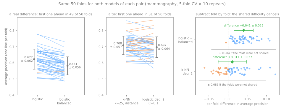
The figure draws one line per fold. On the left the lines are almost parallel and nearly all slope down: whatever makes a fold hard makes it hard for both models, and the balanced one is almost always a little worse. In the middle the lines cross in every direction. On the right, the green bars show the spread of the fold-by-fold difference; the gray bars show what that spread would be if the two models had been scored on unrelated folds (± 0.084 and ± 0.086), between two and three and a half times wider. That is the reason for one cv object with a fixed seed: the comparison becomes paired, and a paired comparison sees differences that two separate mean ± std would hide.
A rule of thumb follows: if the mean difference is smaller than the standard deviation of the per-fold differences, call it a tie. Do not push it further than that. The folds share most of their training rows, so they are not independent measurements, and a textbook paired t-test on them is overconfident. Dietterich (1998) and Nadeau & Bengio (2003) study the problem and propose corrected tests; for choosing a model, the rule of thumb and a look at the figure are enough.
When it is a tie, prefer the simpler model
k-NN and the degree-2 logistic regression are tied. What breaks the tie is everything the metric does not measure. The logistic model is 28 numbers (27 degree-2 features and an intercept) and predicts with one dot product; k-NN carries all 8,946 training rows around and searches them for every prediction. Unless something else matters more, ship the logistic regression. This is Occam's razor, operationalized.
Inside a single family, the classic version of this idea is the one-standard-error rule (Breiman et al., 1984): among the configurations whose mean score is within one standard error of the best, take the simplest. The standard error of a mean over 5 folds is the fold standard deviation divided by \(\sqrt{5}\). For k-NN, a larger k averages more neighbors and gives a smoother, simpler model:
res = pd.DataFrame(searches['k-NN'].cv_results_)
res = res[res['param_kneighborsclassifier__weights'] == 'distance']
table = pd.DataFrame({'k': res['param_kneighborsclassifier__n_neighbors'].to_numpy(),
                      'AP': res['mean_test_score'].to_numpy(),
                      'std': res['std_test_score'].to_numpy()})
best = table['AP'].idxmax()
se = table.loc[best, 'std'] / np.sqrt(5)                # standard error of the best mean
print(table.round(3).to_string(index=False))
print(f"best: k = {table.loc[best, 'k']}, AP {table.loc[best, 'AP']:.3f} · one standard error = {se:.3f}")
print(f"largest k within one SE of the best: {table[table['AP'] >= table.loc[best, 'AP'] - se]['k'].max()}")
  k    AP   std
  5 0.674 0.067
 15 0.707 0.064
 25 0.712 0.054
 35 0.708 0.054
 51 0.693 0.054
 75 0.675 0.052
101 0.662 0.050
best: k = 25, AP 0.712 · one standard error = 0.024
largest k within one SE of the best: 51
The best k is 25 (AP 0.712). Everything above 0.712 − 0.024 = 0.688 is indistinguishable from it, and the simplest configuration in that band is k = 51: twice as many neighbors, for a loss of 0.019 that the one-standard-error convention treats as noise. The C curve in the lab (step 6) uses the looser band of one full standard deviation. Both are conventions for the same advice: do not pay for complexity the data cannot confirm.
The winner's curse, again: nested cross-validation
Stage 3. The winning score, 0.712, is the best of 35 configurations (14 + 7 + 14), each measured on the same folds that were used to pick it. The first section showed where that leads: the best of many noisy estimates is optimistic. To know what the whole procedure ("tune three families, keep the best") is worth on new data, it has to be graded on rows that played no part in it. Nested cross-validation does this with two loops:
from sklearn.base import clone
from sklearn.metrics import average_precision_score

outer = StratifiedKFold(n_splits=5, shuffle=True, random_state=1)
nested, winners = [], []
for tr, va in outer.split(X_dev, y_dev):
    # the complete procedure, on the outer training part only
    fitted = {name: clone(s).fit(X_dev.iloc[tr], y_dev.iloc[tr]) for name, s in searches.items()}
    winner = max(fitted, key=lambda name: fitted[name].best_score_)
    winners.append(winner)
    proba = fitted[winner].predict_proba(X_dev.iloc[va])[:, 1]
    nested.append(average_precision_score(y_dev.iloc[va], proba))
print('winner in each outer fold:', winners)
print(f"best_score_ of the winner: {max(s.best_score_ for s in searches.values()):.3f}")
print(f"nested CV of the choice:   {np.mean(nested):.3f} ± {np.std(nested):.3f}")
winner in each outer fold: ['logistic degree 2', 'k-NN', 'logistic degree 2', 'k-NN', 'logistic degree 2']
best_score_ of the winner: 0.712
nested CV of the choice:   0.702 ± 0.050
Two things come out. The nested estimate, 0.702, is below the 0.712 that the grid search reported. And the winner changes from one outer fold to the next, k-NN in some and the degree-2 logistic in others: the procedure itself cannot tell them apart, which is exactly what the paired comparison said. One nested run is itself noisy, so the figure repeats it with ten different outer shuffles (figure script):
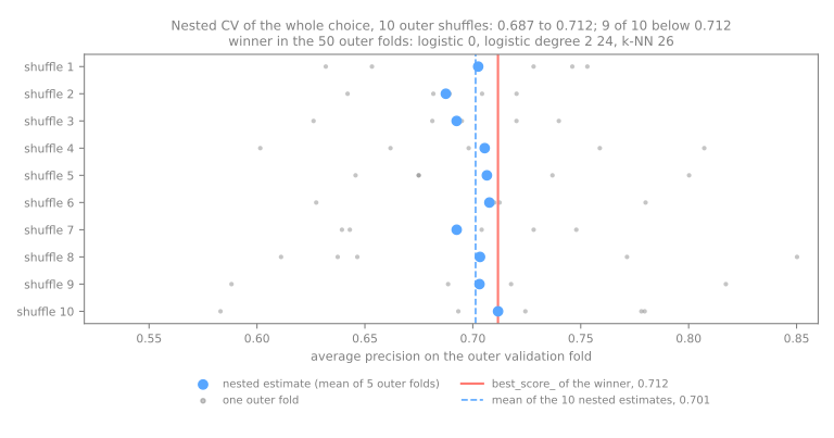
Nine of the ten nested estimates fall below 0.712, the tenth lands on it, and their mean is 0.701. Here the curse costs about one point of AP, because there are only three families and a strong signal; with hundreds of configurations on a small data set it costs far more, as the pure-noise experiment at the top of this lesson showed. Nested CV is expensive (here 5 outer folds × (35 configurations × 5 inner folds + 3 refits of the winners) = 890 fits), and it grades the procedure, not one fitted model: the model you ship is still the procedure run once on all the development data. When there is enough data, the locked test set gives the same protection with a single measurement. Nested CV is for when a test set would be too small to mean anything, or when you want to know how much your own model selection inflates the numbers.
Resampling goes inside the folds
SMOTE, from the ROC and imbalanced data lesson, is a fitted step: it looks at the minority rows and manufactures new ones between neighbors. It therefore belongs inside the pipeline, like the scaler. The tempting shortcut is to oversample the whole table once and then cross-validate:
from imblearn.over_sampling import SMOTE
from imblearn.pipeline import make_pipeline as make_imb_pipeline

knn25 = make_pipeline(StandardScaler(), KNeighborsClassifier(n_neighbors=25, weights='distance'))
scoring = ['average_precision', 'recall', 'precision']

# WRONG: oversample first, then cross-validate on the resampled table
X_res, y_res = SMOTE(random_state=0).fit_resample(X_dev, y_dev)
wrong = cross_validate(knn25, X_res, y_res, cv=cv, scoring=scoring)

# RIGHT: SMOTE is a pipeline step, so in every fold it only sees the training part
smote_knn = make_imb_pipeline(StandardScaler(), SMOTE(random_state=0),
                              KNeighborsClassifier(n_neighbors=25, weights='distance'))
right = cross_validate(smote_knn, X_dev, y_dev, cv=cv, scoring=scoring)
plain = cross_validate(knn25, X_dev, y_dev, cv=cv, scoring=scoring)       # no SMOTE at all

print(f"after SMOTE: {len(y_res)} rows, {y_res.mean():.0%} positive")
for name, r in [('SMOTE before CV', wrong), ('SMOTE in pipeline', right), ('no SMOTE', plain)]:
    print(f"{name:18s}", '  '.join(f"{m} {r['test_' + m].mean():.3f}" for m in scoring))
after SMOTE: 17476 rows, 50% positive
SMOTE before CV    average_precision 0.979  recall 0.963  precision 0.952
SMOTE in pipeline  average_precision 0.601  recall 0.875  precision 0.270
no SMOTE           average_precision 0.712  recall 0.448  precision 0.846
The shortcut reports an AP of 0.979, a model that would be a scientific sensation. Two mistakes add up. A leak: most positives in a validation fold are now synthetic, each one interpolated between two real calcifications that usually sit in the training folds. It is the duplicate-row leak of pattern 3, and k-NN, which predicts from the nearest rows, finds the parents at once. Recall does not depend on how common the positives are, so it shows the leak alone: 0.963 against an honest 0.875. The wrong world: the validation folds are now half positive instead of 2.3% positive, and precision and AP depend on that proportion. A precision of 0.952 measured in a 50/50 world says little about the real one: at 2.3% prevalence there are about forty negatives for every positive, so the same false-alarm rate produces many times more false alarms per hit, and precision falls far below 0.952.
The honest rows also answer the question of the ROC and imbalanced data lesson for this data set. SMOTE in the pipeline raises recall at the default threshold (0.875 against 0.448) by giving up most of the precision (0.270 against 0.846), and it lowers the AP (0.601 against 0.712): the ranking itself got worse. So resampling is one more candidate, to be put in the pipeline, run on the same folds and judged with the same metric as everything else. Here it loses.
Choosing the best model, in order
- Lock the test set away. 2. Choose the metric from the problem. 3. Build every candidate as a pipeline, with every fitted step inside (scaler, encoder, SMOTE). 4. Create one
cvobject with a fixed seed and use it for everything, including aDummyClassifier. 5. Tune each candidate withGridSearchCVon thatcv. 6. Compare the tuned candidates fold by fold; if the mean difference is smaller than the spread of the differences, it is a tie, so take the simpler one. 7. Refit the winner on all the development data and measure it once on the test set, or grade the whole procedure with nested CV.
6. A leak-free experiment, end to end
Stage 4. The complete honest workflow, condensed into a single block, on the breast-cancer dataset — hold-out split, pipeline, stratified CV inside a grid search, one final measurement. The model is a random forest, again a black box here: the recipe does not depend on it.
from sklearn.datasets import load_breast_cancer
from sklearn.model_selection import train_test_split, StratifiedKFold, GridSearchCV
from sklearn.pipeline import Pipeline
from sklearn.preprocessing import StandardScaler
from sklearn.ensemble import RandomForestClassifier
from sklearn.metrics import roc_auc_score

# 1. Final hold-out split (very important!)
X, y = load_breast_cancer(return_X_y=True)
X_train, X_test, y_train, y_test = train_test_split(
    X, y, test_size=0.15, random_state=42, stratify=y)

# 2. Pipeline: every fitted step inside, so CV re-fits it per fold
pipeline = Pipeline([
    ('scaler', StandardScaler()),
    ('clf', RandomForestClassifier(random_state=42)),
])

# 3. Model development: grid search with stratified CV on TRAIN only
cv = StratifiedKFold(n_splits=5, shuffle=True, random_state=42)
param_grid = {
    'clf__n_estimators': [100, 200, 300],
    'clf__max_depth': [5, 10, 20],
}
grid = GridSearchCV(pipeline, param_grid, cv=cv, scoring='roc_auc', n_jobs=-1)
grid.fit(X_train, y_train)
print(grid.best_params_)
print(f"CV ROC AUC of the winner: {grid.best_score_:.4f}")

# 4. The production model: GridSearchCV (refit=True, the default) has already
#    refit the best configuration on ALL of X_train
final_model = grid.best_estimator_

# 5. Honest evaluation — only now, only once
proba = final_model.predict_proba(X_test)[:, 1]
print(f"test ROC AUC:            {roc_auc_score(y_test, proba):.4f}")
{'clf__max_depth': 10, 'clf__n_estimators': 200}
CV ROC AUC of the winner: 0.9923
test ROC AUC:            0.9931
The two numbers agree. That rules out a large optimism from the tuning, but not every leak: a leak that the test set shares (duplicates across the split, the same patient on both sides, a column that encodes the answer) would inflate both numbers alike. Agreement is necessary, not sufficient. Note that grid.best_score_ is the score of the winner of 9 candidates on the folds used to pick it, so the winner's curse says it is slightly optimistic; with 9 candidates and strong signal the bias is invisible here, but with hundreds of candidates on a small dataset it is not. The test score is the one you report. If you need an honest CV estimate of the whole tuning procedure without a test set, wrap the GridSearchCV inside another cross_val_score (nested cross-validation, measured above): the inner loop chooses, the outer loop grades.
7. Exercises
- On the iris dataset, compare K-Fold, Stratified K-Fold, and Leave-One-Out cross-validation: report the mean accuracy for each (and the std of the two k-fold schemes) and explain the differences. Why does the std of the 150 Leave-One-Out scores mean nothing, and why could you not compute recall per Leave-One-Out fold? (Hint:
cross_val_predictpools the predictions.) Then runKFold(3)without shuffling and explain the result (hint: how is iris sorted?). - Using the BOVESPA index (
Closeprices viayfinance, ticker^BVSP, 2 years): useTimeSeriesSplit(5, gap=20)for cross-validation (thegapdrops the 20 days before each validation block, whose targets would reach into it) and fit a linear regression to forecast the index 20 days ahead. Then evaluate the same model with shuffledKFoldand withTimeSeriesSplit(5)without the gap. Which scores are higher, and why are they dishonest? - Rerun the
SelectKBestexperiment withk = 1, 20, 200and with 500, 5,000 and 20,000 noise columns. When is the leak largest? Explain in terms of the winner's curse. - Take the leak-free experiment above, replace
y_trainbynp.random.permutation(y_train)and rerun. What score should you get? Now append 500 columns of pure noise toX_train(np.hstack([X_train, rng.normal(size=(len(X_train), 500))])) and addSelectKBest(k=5)fitted on all of it, with the permuted labels, before the grid search. Compare with the same selector inside the pipeline, for three different permutations. What happens to the permuted-label score? - Redo the model comparison on the mammography data with
scoring='roc_auc'instead of average precision. Does the ranking of the tuned candidates change? Which metric separates them more, and why does that matter when only 2.3% of the rows are positive?
Advanced lab — compare, check and test
Steps 7 to 13 widen the search to two families, compare them fold by fold, check the winner and measure it exactly once on the test set locked away in step 2.
How to run this lab in class (about 35 min, in pairs)
- Use the same Colab notebook as the fundamental lab and go to step 7 (Passo 7). Nothing to download.
- Steps 7 to 13 use the objects of steps 2 to 6 (
X,X_train,X_test,cv,model,dummy). If the Colab session is new (or has expired), click the step 7 cell and use Runtime → Run before (Ctrl+F8) before going on. - Same routine: Predict before running, compare with the page, and try the Simulations before opening the solution.
- Suggested pace: steps 7 and 8 in 10 min; step 9 and its simulation in 12 min; steps 10 and 11 in 8 min; steps 12 and 13 with the simulation in 10 min.
Step 7 — tune the candidates on the same folds
Predict. Each family gets its own grid. Why must both use the same cv object? What would you be measuring if you tuned the logistic regression and left k-NN at its defaults?
from sklearn.neighbors import KNeighborsClassifier

knn = make_pipeline(StandardScaler(), KNeighborsClassifier())
search_lr = GridSearchCV(model, {'logisticregression__C': np.logspace(-3, 3, 13),
                                 'logisticregression__class_weight': [None, 'balanced']},
                         cv=cv, scoring=['recall', 'roc_auc'], refit='recall')
search_knn = GridSearchCV(knn, {'kneighborsclassifier__n_neighbors': [1, 3, 5, 7, 9, 11, 15, 21, 31],
                                'kneighborsclassifier__weights': ['uniform', 'distance']},
                          cv=cv, scoring=['recall', 'roc_auc'], refit='recall')

for name, search in [('logistic', search_lr), ('k-NN', search_knn)]:
    search.fit(X_train, y_train)
    i = search.best_index_
    best_params = ', '.join(f"{k.split('__')[1]}={v:.3g}" if isinstance(v, float) else f"{k.split('__')[1]}={v}"
                            for k, v in search.best_params_.items())
    print(f"{name:8s} {len(search.cv_results_['params'])} configurations · best: {best_params}")
    print(f"{'':8s} recall {search.best_score_:.3f} · ROC AUC {search.cv_results_['mean_test_roc_auc'][i]:.3f}")
logistic 26 configurations · best: C=0.316, class_weight=balanced
         recall 0.959 · ROC AUC 0.995
k-NN     18 configurations · best: n_neighbors=3, weights=uniform
         recall 0.935 · ROC AUC 0.989
Each family gets its own grid, and both grids use the same cv object, so every one of the 44 configurations is scored on the same five folds. scoring lists two metrics: refit='recall' says which one chooses the winner, while ROC AUC is recorded alongside, so a configuration that buys recall by ranking badly would show up.
The logistic grid is the grid of step 6 with class_weight added, and it moves slightly: C = 0.316 with balanced class weights reaches a recall of 0.959, against 0.953 for C = 1 without them. As the ROC and imbalanced data lesson explained, weighting the 37% malignant class more heavily pushes the model toward flagging. k-NN prefers k = 3 and reaches 0.935. That is not yet a verdict: the next two steps check whether these differences are larger than the noise.
Step 8 — compare everything on the same folds
Predict. The tuned logistic regression leads the tuned k-NN by about 0.024 of recall, and the between-fold stds are 0.030 and 0.039. Is that enough to declare a winner?
candidates = {'dummy': dummy,
              'logistic, default': model,
              'logistic, tuned': search_lr.best_estimator_,
              'k-NN, default': knn,
              'k-NN, tuned': search_knn.best_estimator_}
scores = {name: cross_validate(est, X_train, y_train, cv=cv, scoring=['recall', 'roc_auc'])
          for name, est in candidates.items()}
summary = pd.DataFrame({name: {'recall': s['test_recall'].mean(), 'recall std': s['test_recall'].std(),
                               'ROC AUC': s['test_roc_auc'].mean(), 'AUC std': s['test_roc_auc'].std()}
                        for name, s in scores.items()}).T
print(summary.round(3))
                   recall  recall std  ROC AUC  AUC std
dummy               0.000       0.000    0.500    0.000
logistic, default   0.953       0.040    0.996    0.005
logistic, tuned     0.959       0.030    0.995    0.005
k-NN, default       0.918       0.034    0.987    0.014
k-NN, tuned         0.935       0.039    0.989    0.013
One table, one set of folds, five candidates. The dummy is there to anchor the scale: zero recall, ROC AUC 0.5. Tuning seems to help both families a little: k-NN from 0.918 to 0.935, the logistic regression from 0.953 to 0.959. Read those gains with care: each tuned row is scored on the same folds that chose it (the winner's curse again), and 0.953 → 0.959 is a single tumour out of 170. The tuned logistic regression is ahead of the tuned k-NN on both metrics, but look at the standard deviations: 0.030 and 0.039 of recall are larger than the gap between the two tuned models, 0.024. Whether that gap is real is a question for the paired differences.
Step 9 — paired differences, and the winner
Predict. Instead of comparing two means, compare fold by fold. Do you expect the logistic regression to win all five folds, or the sign of the difference to flip?
a, b = scores['logistic, tuned'], scores['k-NN, tuned']
d_recall = a['test_recall'] - b['test_recall']
d_auc = a['test_roc_auc'] - b['test_roc_auc']
print(pd.DataFrame({'recall logistic': a['test_recall'], 'recall k-NN': b['test_recall'],
                    'tumours': np.round(d_recall * 34).astype(int),   # 34 malignant per validation fold
                    'AUC difference': d_auc}).round(3))
for name, d in [('recall', d_recall), ('ROC AUC', d_auc)]:
    print(f"{name:7s} difference: mean {d.mean():+.3f} · std {d.std():.3f} · "
          f"logistic ahead in {(d > 0).sum()} of 5 folds")
   recall logistic  recall k-NN  tumours  AUC difference
0            0.912        0.941       -1          -0.003
1            0.971        1.000       -1          -0.001
2            1.000        0.912        3           0.003
3            0.941        0.882        2           0.020
4            0.971        0.941        1           0.013
recall  difference: mean +0.024 · std 0.047 · logistic ahead in 3 of 5 folds
ROC AUC difference: mean +0.006 · std 0.009 · logistic ahead in 3 of 5 folds
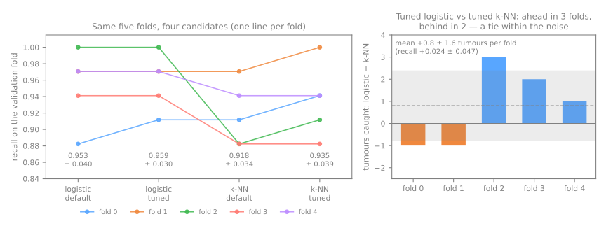
Each validation fold holds 34 malignant tumours, so a difference in recall is a whole number of tumours. The tuned logistic regression catches one tumour fewer than k-NN in folds 0 and 1, and 3, 2 and 1 more in folds 2 to 4: on average 0.8 tumours per fold, with a spread of 1.6. In recall, the mean difference (+0.024) is about half its standard deviation (0.047). By the rule of this lesson, that is a tie. ROC AUC tells the same story: +0.006 ± 0.009.
The rule for picking a winner has to be written down before looking, or it will bend to the result. Ours: the candidate with the better mean recall wins, unless the difference is smaller than the spread of the per-fold differences; in that case break the tie by the second metric, then by simplicity. Here the second metric does not break it either: the ROC AUC difference, +0.006 ± 0.009, is a tie by the same rule. So simplicity decides, and there it is not close: the logistic regression is 31 coefficients instead of 455 stored tumours, its coefficients can be read (step 13), and its probabilities are the raw material for choosing a threshold. The winner is the tuned logistic regression, C = 0.316 with balanced class weights. Its 0.959 is still the best of 26 configurations, so it is slightly optimistic.
Simulation: do more folds change the verdict? Five folds is few. Redo the paired comparison with RepeatedStratifiedKFold(5, n_repeats=10), which gives 50 pairs, and count in how many each model came out ahead. Does the tie of step 9 hold?
Solution
rcv = RepeatedStratifiedKFold(n_splits=5, n_repeats=10, random_state=0)
a = cross_val_score(search_lr.best_estimator_, X_train, y_train, cv=rcv, scoring='recall')
b = cross_val_score(search_knn.best_estimator_, X_train, y_train, cv=rcv, scoring='recall')
d = a - b
print(f"logistic {a.mean():.3f} ± {a.std():.3f}   k-NN {b.mean():.3f} ± {b.std():.3f}")
print(f"paired difference over {len(d)} folds: {d.mean():+.3f} ± {d.std():.3f}")
print(f"logistic ahead in {(d > 0).sum()}, tied in {(d == 0).sum()}, behind in {(d < 0).sum()}")
logistic 0.964 ± 0.029   k-NN 0.935 ± 0.041
paired difference over 50 folds: +0.028 ± 0.030
logistic ahead in 32, tied in 16, behind in 2
With ten times more folds, the mean difference barely moves (+0.028 against +0.024) and is still the size of its own spread: by the lesson's rule of thumb, still a tie. But the count tells a richer story than the rule: across 50 folds the logistic regression was behind in only 2, tied in 16 and ahead in 32. The "mean smaller than the spread = tie" rule is deliberately conservative, because folds share training rows and are not independent measurements. Here it says "do not claim superiority", while the count says "but if you must pick one, there is no reason to prefer k-NN" — which is exactly what step 9 does, breaking the tie on simplicity.
Step 10 — sanity check: shuffle the labels
Predict. With shuffled labels there is nothing to learn. Do you expect recall to fall to zero, to 0.5, or to some other value? (Hint: the winner uses class_weight='balanced'.)
from sklearn.model_selection import permutation_test_score

best = search_lr.best_estimator_                 # the winner of step 9
score, perm_scores, p_value = permutation_test_score(
    best, X_train, y_train, cv=cv, scoring='recall', n_permutations=100, random_state=0)
print(f"real labels: {score:.3f}")
print(f"shuffled labels: mean {perm_scores.mean():.3f}, best of 100 {perm_scores.max():.3f}")
print(f"p-value: {p_value:.4f}")
permutation_test_score reruns the whole cross-validation 100 times with y_train shuffled, which breaks any real link between measurements and diagnosis. With shuffled labels the winner still reaches a recall of 0.480 on average and 0.582 at best. That is not a leak. With balanced class weights and nothing real to learn, the model ends up flagging about half of the rows, and on random labels recall is simply the fraction of rows flagged. "Chance" is a property of the model, not a fixed 50% or 0%, which is why the comparison is made against the shuffled runs. The real labels give 0.959, and the p-value of 0.0099 is the smallest possible with 100 permutations, \(1/101\): not one shuffle came close.
Is it also a leak detector? Much less than it seems. permutation_test_score shuffles y and reruns only what you passed it. A leak that happened before the call (a selector fitted on all the data, duplicate rows, patients spread across folds, a column that encodes the answer) is still there, but the shuffle cuts its link to the new labels: the shuffled scores fall to chance and the p-value approves the leak. Only a step that is rerun with the shuffled labels can show up, which is why the smell test of the leakage section shuffles y at the very start and reruns everything, preprocessing included; even that catches only steps that learn from the labels outside the folds.
Step 11 — out-of-fold predictions
Predict. Why is a confusion matrix built with cross_val_predict honest, while one built with best.predict(X_train) is not?
from sklearn.metrics import confusion_matrix
from sklearn.model_selection import cross_val_predict

oof = cross_val_predict(best, X_train, y_train, cv=cv)      # each row predicted by a model that never saw it
print(confusion_matrix(y_train, oof, labels=[1, 0]))
cross_val_predict returns, for every training row, the prediction made by the fold model that did not train on it. So this confusion matrix is honest: 455 rows, each predicted as unseen data. Out of 170 malignant tumours, 7 were missed (false negatives, top right) and 4 benign ones were flagged (false positives, bottom left). Here the recall stops being an abstract 0.959 and becomes 7 patients. In the ROC and imbalanced data lesson the decision threshold was chosen on a single validation split; out-of-fold probabilities are better material for that choice, because every one of the 455 training rows contributes one honest prediction. The training predictions are not.
Step 12 — the one and only test
Predict. CV said recall 0.959 ± 0.030. Will the test land inside that range? With 42 malignant cases in the test set, how much is one tumour worth in recall points?
from sklearn.metrics import accuracy_score, recall_score, roc_auc_score

pred = best.predict(X_test)                 # GridSearchCV already refit the winner on all of X_train
proba = best.predict_proba(X_test)[:, 1]
print(f"test accuracy {accuracy_score(y_test, pred):.3f} · recall {recall_score(y_test, pred):.3f}"
      f" · ROC AUC {roc_auc_score(y_test, proba):.3f}")
print(confusion_matrix(y_test, pred, labels=[1, 0]))
Once, at the end, the winner meets the locked-away test set. Recall is 0.976 (41 of 42 malignant found, 1 missed), with one false alarm, and ROC AUC is 0.997. That is above the CV estimate of 0.959 ± 0.030, and well inside one standard deviation. With 42 positives, one tumour is worth 2.4 points of recall, so the test set is itself a noisy measurement: the CV told us "about 0.96, give or take 0.03", and the test result agrees.
Note what we did not do: score the runner-up on the test set too. Had we kept whichever of the two did better there, the test set would have become a validation set for the final choice, and its number would carry the winner's curse. Resist the other temptation as well: if a test result disappoints you and you go back to step 7 to try other settings, the test set becomes a validation set and its number stops meaning anything.
Simulation: how much does your own tuning inflate the number? The best_score_ of 0.959 is the best of 26 configurations, measured on the same folds that chose it. Score the logistic search (its 26 configurations) with nested cross-validation — cross_val_score(search_lr, ...) on an outer cv — and compare the three numbers: search, nested CV and test.
Solution
outer = StratifiedKFold(n_splits=5, shuffle=True, random_state=7)
nested = cross_val_score(search_lr, X_train, y_train, cv=outer, scoring='recall')
print(f"best_score_ of the search (chosen on the same folds): {search_lr.best_score_:.3f}")
print(f"nested CV of the logistic search:                   {nested.mean():.3f} ± {nested.std():.3f}")
print(f"recall on the test set:                             {recall_score(y_test, best.predict(X_test)):.3f}")
best_score_ of the search (chosen on the same folds): 0.959
nested CV of the logistic search:                   0.953 ± 0.035
recall on the test set:                             0.976
The nested estimate, 0.953, lands below the 0.959 the search reported. That is consistent with the winner's curse on average, but 0.006 is one tumour out of 170, within the noise of a single nested run, whose outer folds are themselves one random cut. The curse is small here because there are only 26 configurations and the signal is strong; with hundreds of configurations on a small dataset the gap is far larger, as the pure-noise experiment of section 1 showed. The test gave 0.976, above both, a reminder that it too is a noisy measurement: with 42 positives, one tumour is worth 2.4 points. All three numbers sit within one standard deviation of each other: no sign of a large selection bias, although agreement alone cannot rule out a leak that the test set shares. Nested CV scores the procedure; the model that goes to production is still the winner refit on all of X_train.
Step 13 — what did the model learn?
Predict. The features are standardized, so the coefficients are comparable. Do you expect the largest ones to be measures of size, of texture or of shape? And would they be stable if the model were refit on another fold?
coef = pd.Series(best[-1].coef_[0], index=X.columns)
print(coef.sort_values(key=abs, ascending=False).head(6).round(2))
worst texture          0.96
radius error           0.80
worst symmetry         0.72
worst radius           0.68
mean concave points    0.64
worst area             0.64
dtype: float64
Because the pipeline standardizes every feature, the coefficients are on a common scale: each one is the change in the log-odds of malignancy for a one-standard-deviation increase in that measurement. Texture, size and concavity push toward malignant, which is consistent with how pathologists describe these tumours. Read them with care: many of the 30 features are strongly correlated (radius, perimeter and area measure almost the same thing), so the weight can be split between them, and the individual numbers are less stable than the predictions. Fitting the model on each of the five CV training folds (cross_validate(..., return_estimator=True)) shows it: worst texture comes first every time and radius error stays in the top four, while worst symmetry, worst radius, mean concave points and worst concavity trade the remaining places. Treat the list as a hint about what matters, not as a ranking.
To close the class. One sentence each: (1) which of the five leaks can no CV scheme catch? (2) Why does comparing fold by fold see differences that two mean ± std hide? (3) Why is the best_score_ of a grid search optimistic?
Your turn (advanced)
For homework, with more time:
- Threshold. Use
cross_val_predict(best, X_train, y_train, cv=cv, method='predict_proba')[:, 1]to get out-of-fold probabilities. Find the highest threshold that gives recall ≥ 0.98 and report the precision you pay for it. Then apply that threshold, once, to the test set. - L1 penalty. Switch to
LogisticRegression(l1_ratio=1, solver='liblinear')(on scikit-learn before 1.8, writepenalty='l1') and repeat step 6. How many of the 30 coefficients are exactly zero at the bestC? Does recall change by more than one standard deviation? - The whole choice, nested. The step 12 simulation nested only the logistic search. Write the outer loop yourself, as in the nested CV section, so that it scores steps 7 to 9 together: both searches and the choice between them. Does the number drop further?
- More candidates. Add a SMOTE + k-NN candidate to the step 8 table (an
imblearnpipeline, as in the ROC and imbalanced data lesson) tuned on the samecvand compare it with the winner fold by fold. After the SVM lesson, come back and add anSVCtoo. Does any of them beat the tuned logistic regression by more than the spread of the paired differences?
References
- Stone, M. "Cross-Validatory Choice and Assessment of Statistical Predictions." JRSS B 36 (1974). DOI
- Ambroise, C.; McLachlan, G. J. "Selection Bias in Gene Extraction on the Basis of Microarray Gene-Expression Data." PNAS 99, no. 10 (2002): 6562–6566 — feature selection before cross-validation, found in published work. DOI
- Cawley, G. C.; Talbot, N. L. C. "On Over-fitting in Model Selection and Subsequent Selection Bias in Performance Evaluation." JMLR 11 (2010): 2079–2107 — the winner's curse in model selection, and nested CV. PDF
- Kaufman, S.; Rosset, S.; Perlich, C.; Stitelman, O. "Leakage in Data Mining: Formulation, Detection, and Avoidance." ACM TKDD 6, no. 4 (2012) — a taxonomy of leakage with real competition cases. DOI
- Breiman, L.; Friedman, J. H.; Olshen, R. A.; Stone, C. J. Classification and Regression Trees. Wadsworth (1984) — where the one-standard-error rule comes from. DOI
- Dietterich, T. G. "Approximate Statistical Tests for Comparing Supervised Classification Learning Algorithms." Neural Computation 10, no. 7 (1998): 1895–1923 — why tests on cross-validation folds are overconfident. DOI
- Nadeau, C.; Bengio, Y. "Inference for the Generalization Error." Machine Learning 52 (2003): 239–281 — the corrected test for comparing models on CV folds. DOI
- Moscovich, A.; Rosset, S. "On the Cross-Validation Bias due to Unsupervised Preprocessing." JRSS B 84, no. 4 (2022): 1474–1502 — fitting a step that ignores the labels on all the data biases CV, usually a little and in either direction. DOI
- Chawla, N. V.; Bowyer, K. W.; Hall, L. O.; Kegelmeyer, W. P. "SMOTE: Synthetic Minority Over-sampling Technique." JAIR 16 (2002): 321–357 — SMOTE, introduced on several data sets, including the mammography data used in this lesson (OpenML 310). DOI
Quiz
The quiz covers the fundamental approach.