Machine Learning · Insper

Leakage and Comparison

Advanced approach

How your estimate can lie — and how not to fool yourself

The path of this part

Find the leaksfive patterns, each one measured; the smell test
Compare fairlymetric first, tuned candidates, same folds, ties
Grade the winnernested cross-validation (CV), resampling inside the folds
End to endthe steps in order, then the lab: compare, check and test

Each stage answers one question: where can information sneak into training? → is one candidate really better? → how optimistic is the winner's score? → what does an honest experiment look like, start to finish?

Stage 1 · Where can information sneak into training?

Leakage = information from outside the training fold

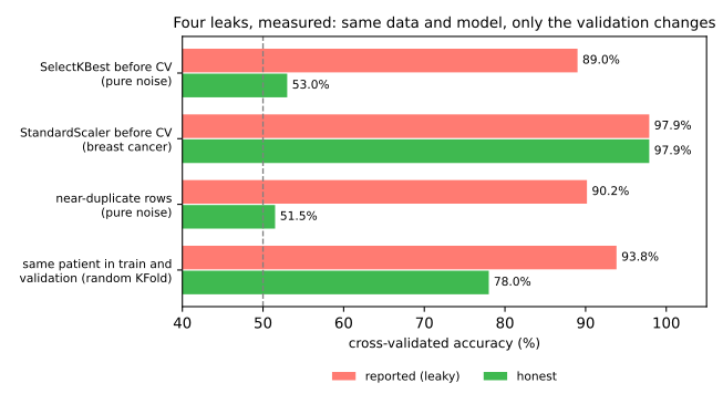
Reported vs honest accuracy for four leaks

Four classic patterns, each measured twice on the same data: once with the leak, once with honest validation.

The model looks brilliant in evaluation and collapses in production, where the leaked information does not exist yet.

1. Preprocessing before the split

Predict. 100 rows, 5,000 columns of pure noise, coin-flip labels. The selector keeps 20 columns looking at all 100 labels, then CV runs. What accuracy comes out? And with the selector inside the pipeline?


# WRONG: the selector sees all 100 labels, then CV runs on the surviving columns
X_sel = SelectKBest(f_classif, k=20).fit_transform(X, y)
cross_val_score(LogisticRegression(), X_sel, y, cv=cv).mean()   # 0.89

# RIGHT: the selector is refit inside each fold
pipe = make_pipeline(SelectKBest(f_classif, k=20), LogisticRegression())
cross_val_score(pipe, X, y, cv=cv).mean()                       # 0.53

89% on data with no signal at all. Among 5,000 random columns, some correlate with the labels by chance — including the labels of the rows that will later be validation.

A StandardScaler making the same mistake changes almost nothing (97.9% either way). The size of a leak depends on what the step learns — and you cannot know without measuring. The pipeline makes the question disappear.

Simulator: leakage on pure noise

Predict. Nothing here is learnable: an honest pipeline must land at 50%. Raise the noise features from 20 to 300: what happens to the reported score, and to the honest one?

2 and 3. The future and the duplicates

Predict. Each row gets a near-identical twin; the labels are coin flips. What accuracy will 1-NN (k-nearest neighbors, k-NN, with \(k = 1\)) report under shuffled KFold? Can you get it by hand?

Features that know the future

Predicting readmission with number_of_followup_visits; predicting churn with account_closed_date is null.

No CV scheme catches this: the leak is in the columns, not in the split. Ask of every feature: does this value exist at prediction time?

Duplicated rows

1-NN, original data	0.487
with twins, KFold	0.902
with twins, GroupKFold	0.515

The twin lands in training with probability 4/5; 1-NN finds it: \(0.8 \times 1 + 0.2 \times 0.5 = 0.9\).

4 and 5. Groups and time

Predict. Will random KFold score above or below 200 brand-new patients? And what R² (coefficient of determination) should an honest split give on a random walk?

Group leakage

60 patients, 10 scans each; each patient has a "fingerprint".

random KFold	0.938
GroupKFold by patient	0.780
200 new patients	0.7545

The model recognizes the patient, not the disease. The grouped estimate was the honest one.

Temporal leakage

A random walk; the only feature is the day number:

shuffled KFold	R² 0.99
TimeSeriesSplit	R² −1.78

Every validation day is surrounded by training days: that is interpolation, which production never offers. The −1.78 is the correct answer: the best honest forecast, “tomorrow = last value seen”, scores −1.70.

Always ask: what is the unit I will predict on in production? Make that the unit of the split.

The smell test

Results that look too good — 99% on a hard problem, a feature with implausible importance, a huge gap between offline and production — suspect leakage first, not genius.
Run the cheapest test there is: shuffle y at the very start and rerun the whole pipeline, preprocessing included. The score must fall to the shuffled baseline (chance for that model and metric, not necessarily 50%).

If it does not, some step learns from the labels outside the folds, like a selector fitted before CV.

Passing proves less: duplicates, groups, time order and leaked columns lose their link to the shuffled labels too, so leaks 2 to 5 pass this test anyway.

Stage 2 · Is one candidate really better?

Comparing models: six rules

choose the metric from the problem, before looking at any model;
tune every candidate before comparing them;
score them all on the same folds and compare fold by fold;
when two are within the noise, prefer the simpler one;
the winner's score is optimistic: score the whole choice;
resampling happens inside the folds.

Rule 2, measured in average precision (AP, next slide): at their defaults, the degree-2 logistic beat k-NN by 0.087. Tuned, the gap vanishes (0.712 against 0.711). The default k = 5 was simply a bad choice.

Choose the metric first

Mammography: 11,183 regions of mammograms, 6 numbers each; only 2.3% are calcifications. Five candidates, the same 5 folds, mean over folds.

Predict. What accuracy does a dummy that never flags anything get?

	accuracy	ROC AUC	AP
dummy (never flags)	0.977	0.500	0.023
logistic	0.983	0.923	0.622
logistic balanced	0.901	0.921	0.585
logistic degree 2	0.986	0.948	0.710
k-NN	0.986	0.904	0.623

ROC AUC: area under the ROC (receiver operating characteristic) curve. AP (average precision): area under the precision–recall curve; a random ranking gets the prevalence.

Accuracy cannot separate them; ROC AUC squeezes the real models into 0.90–0.95; AP separates them (0.023 to 0.710). Pick the metric from the problem, before looking.

Compare fold by fold

Predict. Logistic 0.622 ± 0.050 against balanced 0.585 ± 0.048: is that a tie? What changes if you subtract fold by fold?

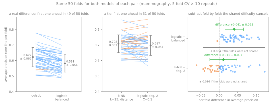
Logistic beats balanced logistic in 49 of 50 folds although their means overlap; k-NN and degree 2 swap places

	difference	ahead
logistic − balanced	+0.041 ± 0.025	49/50
k-NN − degree 2	+0.011 ± 0.037	31/50

The first pair looks like a tie by mean ± std (0.622 ± 0.050 against 0.585 ± 0.048). Fold by fold, there is no tie at all: subtracting cancels the fold's shared difficulty.

Rule of thumb: if the mean difference is smaller than the std of the per-fold differences, call it a tie. Folds share training rows, so a textbook paired t-test is overconfident.

Tied? Prefer the simpler one

The one-standard-error rule (Breiman et al., 1984) on k-NN (\(k\) = number of neighbors):

k	AP
25	0.712
35	0.708
51	0.693
75	0.675

Std of the 5 fold scores at \(k = 25\): 0.054, so one standard error \(= 0.054/\sqrt{5} = 0.024\); band: AP \(\geq 0.712 - 0.024 = 0.688\). The largest \(k\) inside it is 51.

And between tied families, what breaks the tie is what the metric does not measure:

the degree-2 logistic is 28 numbers and a dot product;
k-NN carries the 8,946 training rows and walks them at every prediction.

Occam's razor, operationalized: do not pay for complexity the data cannot confirm.

Stage 3 · How optimistic is the winner's score?

Nested cross-validation: two loops

The winner, 0.712, is the best of 35 configurations measured on the folds that chose it. To know what the whole procedure is worth, grade it on rows that played no part in it.

The winner's curse, again

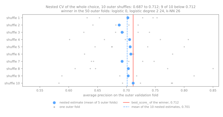
Ten nested CV estimates run from 0.687 to 0.712, nine of them below the best_score_ of 0.712

Predict. Will the nested estimate land above, on or below 0.712? Will the same family win in every outer fold?

Nested CV runs the whole choice inside each outer fold and scores outside it: 0.702 ± 0.050.
The winner changes from outer fold to outer fold — the procedure cannot tell the families apart.

Nested CV scores the procedure, not a model. It is expensive (890 fits here); with enough data, a locked test set gives the same protection with one measurement.

Resampling goes inside the folds

Predict. SMOTE (Synthetic Minority Over-sampling Technique) creates new positives between neighboring ones. Applied to the whole table before CV, does AP go up or down? And inside the pipeline?

	AP	recall	precision
SMOTE before CV	0.979	0.963	0.952
SMOTE in the pipeline	0.601	0.875	0.270
no SMOTE	0.712	0.448	0.846

A leak: most validation positives are now synthetic, interpolated between calcifications that sit in training;
The wrong world: the validation folds became 50% positive instead of 2.3%, and precision and AP depend on that.

Resampling is just another candidate: in the pipeline, on the same folds, judged by the same metric. Here it loses — AP falls from 0.712 to 0.601.

Stage 4 · What does an honest experiment look like, start to finish?

Choosing the best model, in order

Lock the test set away.
Choose the metric from the problem.
Build each candidate as a pipeline, with every fitted step inside.
Create one cv object with a fixed seed and use it for everything, including the DummyClassifier.
Tune each candidate with GridSearchCV on that cv.
Compare fold by fold; difference smaller than the spread = tie, keep the simpler one.
Refit the winner and measure it once on the test set, or score the procedure with nested CV.

A leak-free experiment, end to end

Breast cancer, a random forest, a grid of 9 configurations; 15% locked away as the test set before anything else.


X_train, X_test, y_train, y_test = train_test_split(
    X, y, test_size=0.15, random_state=42, stratify=y)
pipeline = Pipeline([('scaler', StandardScaler()),
                     ('clf', RandomForestClassifier(random_state=42))])
grid = GridSearchCV(pipeline, param_grid, cv=cv, scoring='roc_auc')
grid.fit(X_train, y_train)                      # CV on the training part only
proba = grid.best_estimator_.predict_proba(X_test)[:, 1]   # the test, once

Predict. The CV score is the best of 9 configurations. Will the test score land far below it?

CV ROC AUC of the winner (`grid.best_score_`)	0.9923
test ROC AUC, measured once	0.9931

They agree: no sign of a large optimism from the tuning. Agreement is necessary, not sufficient: a leak the test set shares (duplicates across the split, the same patient on both sides, a leaked column) would inflate both alike.

Advanced lab · about 35 min, in pairs

Compare, check and test: steps 7 to 13

Same Colab notebook, from step 7 (Passo 7). New session? Runtime → Run before.
Two families tuned on the same folds, compared fold by fold, with a tie-break rule written before looking.
Simulations: do more folds change the verdict? (step 9) and how much does your own tuning inflate the number? (step 12).
Steps 10 and 11: shuffling the labels and out-of-fold predictions.

Pace: steps 7 and 8 in 10 min; step 9 and its simulation in 12 min; steps 10 and 11 in 8 min; steps 12 and 13 with the simulation in 10 min.