Agrupamento
Boa parte do aprendizado de máquina — os modelos supervisionados, que vêm mais adiante no curso — precisa de alguém dizendo o que cada linha é: um rótulo para cada exemplo. O agrupamento (clustering) dispensa isso: recebe só a tabela \(X\) (sem rótulos) e devolve uma partição das linhas em grupos cujos membros se parecem entre si e diferem dos membros dos outros grupos. Estrutura é de graça e rótulo é caro; é por isso que o agrupamento aparece em toda parte: segmentar clientes, comprimir imagens (uma paleta de \(k\) cores é um agrupamento dos pixels), apontar linhas que não se parecem com nada, rotular um representante por grupo em vez de cada linha e organizar documentos (o caminho até a modelagem de tópicos).
O preço de não ter rótulos é não ter gabarito. O algoritmo sempre devolve uma partição, haja ou não grupos nos dados; se ela é boa depende de critérios que você escolhe. Esta aula trata de um algoritmo para cada ideia do que é um grupo (k-means: pontos perto de um centro; DBSCAN e HDBSCAN: regiões densas separadas por regiões esparsas) e, na mesma medida, dos números usados para julgá-los e do que esses números não conseguem dizer.
Todo número abaixo é medido: os blocos de código o imprimem e cada figura é produzida por um script curto que fica ao lado desta página.
A aula segue um pipeline em cinco etapas, desenhado abaixo: 1. definir e julgar, o que significa "parecido" e como se dá nota a uma partição; 2. k-means, o algoritmo de Lloyd feito à mão; 3. escolher k, com o cotovelo, a silhueta e o que eles não conseguem dizer; 4. além dos centros, onde o k-means falha e como o DBSCAN e o HDBSCAN acham regiões densas no lugar de centros; 5. escolher e interpretar, decidir o algoritmo e dizer o que é cada grupo. Cada etapa leva à sua seção; nos slides, uma faixa embaixo mostra em que etapa você está.
- Definir e julgardistância, índices internos e externos
- k-meanso algoritmo de Lloyd à mão, mínimos locais
- Escolher kcotovelo, silhueta, outros índices, escala
- Além dos centrosonde o k-means falha; DBSCAN, HDBSCAN
- Escolher e interpretarqual algoritmo, o que é cada grupo
Slides
Clique nos slides e use as setas ← → para navegar; F abre em tela cheia e Esc mostra todos os slides. Abrir os slides numa aba nova
O que é agrupar e como se julga um agrupamento
| Classificação | Agrupamento | |
|---|---|---|
| entrada | \(X\) e \(y\) | só \(X\) |
| "acertar" é | prever \(y\) em linhas novas | satisfazer um critério que você escolheu |
| validado com | um conjunto de teste separado | sem rótulos, não há conjunto de teste possível |
Etapa 1. Duas decisões vêm antes de qualquer algoritmo:
- O que "parecido" significa. Quase todo método de agrupamento trabalha com distâncias, em geral euclidianas. Uma distância soma diferenças entre colunas, então uma coluna medida em gramas afoga outra medida em milímetros. Escalonar (Pré-processamento) faz parte do agrupamento; a seção A escala importa mede quanto.
- Como o resultado será julgado. Há duas famílias de índices:
- índices internos usam só \(X\) e a partição: a inércia, a silhueta, Calinski–Harabasz, Davies–Bouldin. Num projeto real, são tudo o que você tem;
- índices externos comparam a partição com rótulos conhecidos. O padrão é o Índice de Rand Ajustado (ARI, Adjusted Rand Index; Hubert & Arabie, 1985). Num problema não supervisionado de verdade não há rótulos, então o ARI não pode ser usado para escolher nada; ele é usado aqui, em dados cujos grupos verdadeiros por acaso conhecemos, para conferir se os índices internos apontam na direção certa.
O ARI olha para cada par de pontos e pergunta se as duas partições concordam sobre ele: ambas põem o par junto ou ambas o mantêm separado. A fração de pares com concordância é o índice de Rand. Tome seis pontos cujos grupos verdadeiros são \(\{1,2,3\}\) e \(\{4,5,6\}\); um agrupamento os divide em \(\{1,2\}, \{3,4\}, \{5,6\}\). Dos 15 pares, as duas partições concordam em 10: dois pares juntos nas duas — (1,2) e (5,6) — e oito pares separados nas duas: os nove pares cruzados menos o (3,4). O índice de Rand é então \(10/15 = 0{,}667\). Mas rótulos aleatórios também concordam em muitos pares (a maioria dos pares está "separada" nas duas), então o ARI desconta o que o acaso daria e reescala: 1 para partições idênticas, perto de 0 para partições aleatórias.
import numpy as np
from sklearn.metrics import adjusted_rand_score, rand_score

truth = [0, 0, 0, 1, 1, 1]
print(adjusted_rand_score(truth, [1, 1, 1, 0, 0, 0]))            # mesmos grupos, nomes trocados
print(round(rand_score(truth, [0, 0, 1, 1, 2, 2]), 3),
      round(adjusted_rand_score(truth, [0, 0, 1, 1, 2, 2]), 3))  # o exemplo acima
rng = np.random.default_rng(0)
print(round(adjusted_rand_score(rng.integers(0, 3, 1000), rng.integers(0, 3, 1000)), 3))  # acaso
A primeira linha mostra por que a acurácia não serve: um agrupamento não sabe qual grupo é o "0", então uma partição perfeita pode vir com os nomes trocados; o ARI ignora nomes. A segunda confirma a contagem à mão (índice de Rand 0,667) e mostra a correção do acaso baixando-o para um ARI de 0,242. A terceira é o que obtêm duas partições de 1.000 pontos sem relação entre si: praticamente zero.
k-means
Etapa 2. O k-means (Lloyd, 1982; MacQueen, 1967) diz que um grupo é o conjunto dos pontos mais próximos de um centro. Você escolhe \(k\); ele procura \(k\) centros \(\mu_1, \dots, \mu_k\) e uma atribuição de pontos a eles que minimizem a inércia, também chamada de soma dos quadrados intragrupo (WCSS, within-cluster sum of squares):
Em palavras: a soma, sobre todos os pontos, do quadrado da distância ao centro do próprio grupo, sendo cada centro a média do seu grupo. A fórmula é circular: os centros dependem de quem está em cada grupo; quem está em cada grupo depende de qual centro está mais perto. O algoritmo de Lloyd quebra o círculo alternando as duas metades até nada mudar:
- atribuir: cada ponto vai para o centro mais próximo;
- atualizar: cada centro vai para a média dos pontos que recebeu.
Nenhum dos passos pode aumentar \(J\). Mandar um ponto para o centro mais próximo só pode encurtar a sua parcela; já a média é exatamente o ponto que minimiza a soma dos quadrados das distâncias a um conjunto de pontos. Como \(J\) nunca sobe e o número de partições é finito, o algoritmo sempre para. Isso não quer dizer que ele pare na melhor partição, como Inicialização vai mostrar.
O algoritmo de Lloyd, à mão
Oito pontos e \(k = 2\). Dois quadrados de lado 1, um em torno de \((1{,}5;\ 1{,}5)\) e outro em torno de \((6{,}5;\ 5{,}5)\). O começo é ruim de propósito: os dois centros dentro do quadrado da esquerda, \(c_1 = (1, 1)\) e \(c_2 = (2, 2)\). Distâncias ao quadrado dispensam raízes.
| ponto | coordenadas | \(d^2\) a \(c_1=(1,1)\) | \(d^2\) a \(c_2=(2,2)\) | grupo | \(d^2\) a \((4/3;\ 4/3)\) | \(d^2\) a \((5{,}6;\ 4{,}8)\) | grupo |
|---|---|---|---|---|---|---|---|
| \(x_1\) | (1, 1) | 0 | 2 | 1 | 0,22 | 35,60 | 1 |
| \(x_2\) | (2, 1) | 1 | 1 | 1 | 0,56 | 27,40 | 1 |
| \(x_3\) | (1, 2) | 1 | 1 | 1 | 0,56 | 29,00 | 1 |
| \(x_4\) | (2, 2) | 2 | 0 | 2 | 0,89 | 20,80 | 1 |
| \(x_5\) | (6, 5) | 41 | 25 | 2 | 35,22 | 0,20 | 2 |
| \(x_6\) | (7, 5) | 52 | 34 | 2 | 45,56 | 2,00 | 2 |
| \(x_7\) | (6, 6) | 50 | 32 | 2 | 43,56 | 1,60 | 2 |
| \(x_8\) | (7, 6) | 61 | 41 | 2 | 53,89 | 3,40 | 2 |
| inércia | 134 | 9,42 |
- Iteração 0, atribuir. \(x_2\) e \(x_3\) empatam (distância 1 aos dois); o empate vai para o primeiro centro. \(x_4\) está exatamente sobre \(c_2\), então entra no grupo 2, junto com os quatro pontos a seis unidades de distância. A inércia é \(0+1+1+0+25+34+32+41 = 134\). O algoritmo acabou de cometer um erro e nada nele percebe.
- Iteração 0, atualizar. \(c_1\) = média de \(x_1, x_2, x_3\) = \(\big(\tfrac{1+2+1}{3}; \tfrac{1+1+2}{3}\big) = (4/3;\ 4/3)\). \(c_2\) = média de \(x_4, \dots, x_8\) = \(\big(\tfrac{28}{5}; \tfrac{24}{5}\big) = (5{,}6;\ 4{,}8)\).
- Iteração 1, atribuir (metade direita da tabela). Com \(c_2\) arrastado para a direita, \(x_4\) fica muito mais perto de \(c_1\) (0,89 contra 20,80) e volta. A inércia cai para 9,42. Atualizar: \(c_1 = (1{,}5;\ 1{,}5)\), \(c_2 = (6{,}5;\ 5{,}5)\).
- Iteração 2. Todo ponto está a \(d^2 = 0{,}5\) do centro do seu quadrado, então a inércia é \(8 \times 0{,}5 = 4{,}00\). Nenhuma atribuição muda, os centros não se movem: convergiu.
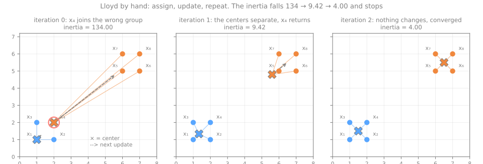
Três coisas que a tabela mostra e a fórmula não. A inércia cai rápido (134 → 9,42 → 4,00): a primeira iteração faz quase todo o trabalho, como costuma acontecer. Uma atribuição errada de um ponto se corrige sozinha quando os centros se movem. E convergir é um teste de igualdade, "nenhuma atribuição mudou", não uma tolerância. O mesmo laço em NumPy, imprimindo cada iteração:
X = np.array([[1, 1], [2, 1], [1, 2], [2, 2], [6, 5], [7, 5], [6, 6], [7, 6]], dtype=float)
C = np.array([[1, 1], [2, 2]], dtype=float)                    # o começo ruim

for it in range(10):
    d2 = ((X[:, None, :] - C[None, :, :]) ** 2).sum(axis=2)     # distâncias ao quadrado, 8 pontos x 2 centros
    labels = d2.argmin(axis=1)                                   # 1. atribuir (empate vai para o primeiro centro)
    inertia = d2[np.arange(len(X)), labels].sum()
    C_new = np.array([X[labels == j].mean(axis=0) for j in range(2)])   # 2. atualizar
    print(f"iteration {it}: groups {labels}  inertia {inertia:6.2f}  new centers {C_new.round(3).tolist()}")
    if np.allclose(C_new, C):                                    # nada se moveu: convergiu
        break
    C = C_new
iteration 0: groups [0 0 0 1 1 1 1 1]  inertia 134.00  new centers [[1.333, 1.333], [5.6, 4.8]]
iteration 1: groups [0 0 0 0 1 1 1 1]  inertia   9.42  new centers [[1.5, 1.5], [6.5, 5.5]]
iteration 2: groups [0 0 0 0 1 1 1 1]  inertia   4.00  new centers [[1.5, 1.5], [6.5, 5.5]]
O scikit-learn, partindo dos mesmos dois centros, chega à mesma partição:
from sklearn.cluster import KMeans

km = KMeans(n_clusters=2, init=np.array([[1, 1], [2, 2]]), n_init=1).fit(X)
print(km.labels_, km.cluster_centers_.tolist(), km.inertia_)
Execute as mesmas duas operações, passo a passo, numa nuvem maior. Os traços ligam cada ponto ao seu centro; a inércia é a soma dos quadrados dos seus comprimentos; o histórico dela, à direita, nunca sobe:
Por que a média e não outro ponto qualquer
O passo de atualização põe cada centro na média do seu grupo porque a média é o ponto que minimiza a soma dos quadrados das distâncias àquele grupo: é a definição do critério, não uma convenção. Tente vencê-la à mão: arraste os centros, veja qual grupo contribui mais para a inércia e depois aperte o botão que leva cada centro à sua média. Quando as setas somem, o algoritmo convergiu.
Inicialização e mínimos locais
O algoritmo de Lloyd para na primeira partição da qual nenhum dos dois passos consegue melhorar. Isso é um mínimo local da inércia; qual deles você alcança depende de onde os centros começaram. Tome 300 pontos em três bolhas bem separadas e rode o k-means com um começo por execução (n_init=1), 100 vezes com sementes diferentes, uma vez com centros iniciais sorteados e outra com o k-means++ (Arthur & Vassilvitskii, 2007). O k-means++ sorteia o primeiro centro entre os pontos e cada um dos seguintes com probabilidade proporcional ao quadrado da distância ao centro mais próximo já escolhido, de modo que os centros iniciais tendem a ficar espalhados.
from sklearn.datasets import make_blobs

X_blobs, _ = make_blobs(n_samples=300, centers=3, cluster_std=1.0, random_state=42)
for init in ['random', 'k-means++']:
    inertias = np.array([KMeans(n_clusters=3, init=init, n_init=1, random_state=s).fit(X_blobs).inertia_
                         for s in range(100)])
    stuck = (inertias > 1.01 * inertias.min()).sum()
    print(f"{init:10s} best {inertias.min():7.1f}  worst {inertias.max():7.1f}  stuck in {stuck} of 100 runs")

worst = max(KMeans(n_clusters=3, init='random', n_init=10, random_state=s).fit(X_blobs).inertia_
            for s in range(100))
print(f"random init, n_init=10: worst of 100 runs {worst:.1f}")
random     best   566.9  worst  5703.3  stuck in 22 of 100 runs
k-means++  best   566.9  worst   566.9  stuck in 0 of 100 runs
random init, n_init=10: worst of 100 runs 566.9
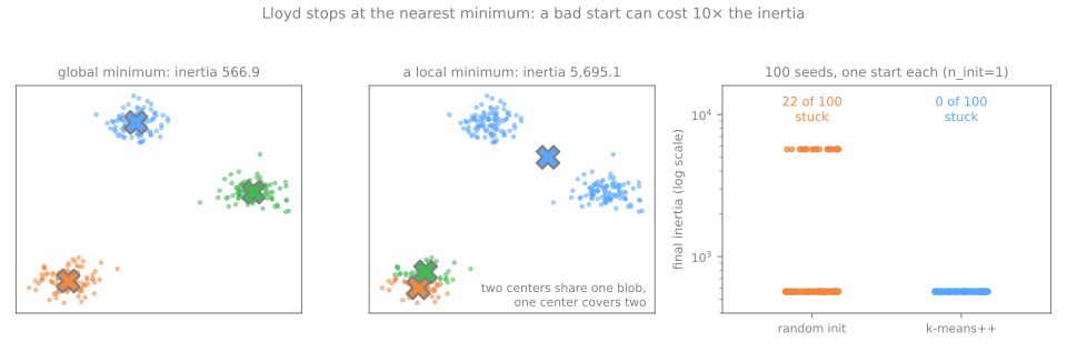
Com centros iniciais sorteados, 22 execuções em 100 convergem para uma inércia dez vezes maior que a melhor: dois centros dividem uma bolha e o terceiro fica entre as outras duas; nenhum dos passos conserta isso, porque mover um único centro ou um único ponto piora a inércia. É um erro que envolve centros inteiros e, ao contrário do \(x_4\) do exemplo à mão, não se corrige sozinho. O k-means++ nunca ficou preso aqui. A regra prática é a que o scikit-learn segue: n_init reinicia o algoritmo inteiro a partir de várias inicializações e fica com a de menor inércia; com n_init=10, nem os começos sorteados perderam em 100 execuções. O k-means++ é o init padrão do scikit-learn; o padrão n_init='auto' significa uma única execução com k-means++ (dez com começos sorteados). Esta aula escreve n_init=10 explicitamente.
Escolhendo k
Etapa 3. A inércia é o que o k-means minimiza, então ela não pode escolher \(k\): acrescentar um centro só pode baixá-la; com \(k = n\), cada ponto é o seu próprio centro e a inércia é 0. Escolher \(k\) exige critérios que não melhoram automaticamente com mais grupos.
O cotovelo
Desenhe a inércia contra \(k\) e procure o cotovelo, o \(k\) a partir do qual acrescentar um grupo rende bem menos do que antes. É uma heurística muitas vezes ambígua, aplicada a uma curva que sempre desce.
A silhueta, à mão
A silhueta (Rousseeuw, 1987) pergunta a cada ponto: você está melhor no seu grupo do que estaria no grupo vizinho?
em que \(a(i)\) é a distância média do ponto \(i\) aos outros pontos do próprio grupo e \(b(i)\), a distância média aos pontos do grupo vizinho mais próximo. \(s\) perto de 1: bem instalado no seu grupo; perto de 0: na fronteira; negativo: mais perto, em média, de outro grupo. A silhueta de um agrupamento é a média de \(s(i)\) sobre todos os pontos. Ela usa distâncias simples, não ao quadrado.
De volta aos oito pontos, na partição final \(\{x_1..x_4\}\), \(\{x_5..x_8\}\). Para \(x_1 = (1,1)\):
- \(a(x_1)\): as distâncias a \(x_2, x_3, x_4\) são \(1, 1, \sqrt2\), então \(a = (1 + 1 + 1{,}414)/3 = 1{,}1381\);
- \(b(x_1)\): as distâncias a \(x_5..x_8\) são \(\sqrt{41}, \sqrt{52}, \sqrt{50}, \sqrt{61}\) = 6,403; 7,211; 7,071; 7,810, então \(b = 7{,}1239\);
- \(s(x_1) = (7{,}1239 - 1{,}1381) / 7{,}1239 = 0{,}8402\).
from sklearn.metrics import silhouette_samples, silhouette_score

labels = np.array([0, 0, 0, 0, 1, 1, 1, 1])                        # a partição final
D = np.sqrt(((X[:, None, :] - X[None, :, :]) ** 2).sum(axis=2))   # distâncias euclidianas
a, b = D[0, 1:4].mean(), D[0, 4:8].mean()                          # x1 ao seu grupo, x1 ao outro
print(f"a = {a:.4f}  b = {b:.4f}  s = {(b - a) / max(a, b):.4f}")
print(silhouette_samples(X, labels).round(4))
print(round(silhouette_score(X, labels), 4))
A biblioteca confirma \(s(x_1) = 0{,}8402\). Os oito valores também dizem algo que a média esconde: \(a\) é o mesmo, 1,1381, para todos os pontos (de qualquer vértice de um quadrado de lado 1, os outros três estão a 1, 1 e \(\sqrt2\)), então só \(b\) os ordena. Os vértices de fora, \(x_1\) e \(x_8\), são os mais distantes do outro quadrado e têm a maior silhueta; os de dentro, \(x_4\) e \(x_5\), têm a menor, 0,8011. A média, 0,8223, é altíssima, como deve ser para dois quadradinhos a cinco unidades de distância. Clique em qualquer ponto do simulador para ver os seus dois círculos, \(a\) na cor do próprio grupo e \(b\) na do vizinho; as barras à direita são a silhueta de todos os pontos, ordenadas por grupo, que é como se lê um agrupamento inteiro de uma vez:
Mais dois índices internos
O scikit-learn oferece mais dois índices feitos dos mesmos ingredientes, coesão contra separação:
- Calinski–Harabasz (Caliński & Harabasz, 1974), quanto maior melhor: a razão entre a dispersão entre grupos e a dispersão dentro dos grupos, cada uma dividida pelos seus graus de liberdade, \(\mathrm{CH} = \dfrac{B/(k-1)}{W/(n-k)}\), com \(W\) a inércia e \(B = \sum_j |C_j|\,\lVert \mu_j - \bar x \rVert^2\);
- Davies–Bouldin (Davies & Bouldin, 1979), quanto menor melhor: para cada grupo, tome o seu pior vizinho, aquele que maximiza \((s_i + s_j)/d(\mu_i, \mu_j)\), em que \(s_i\) é a distância média dos pontos do grupo \(i\) ao seu centro; depois tire a média sobre os grupos.
Nos oito pontos, à mão: a média geral é \(\bar x = (4;\ 3{,}5)\); cada centro está a uma distância ao quadrado de \(2{,}5^2 + 2^2 = 10{,}25\) dela, então \(B = 4 \times 10{,}25 + 4 \times 10{,}25 = 82\), \(W = 4\) e \(\mathrm{CH} = (82/1)/(4/6) = 123\). Cada ponto está a \(\sqrt{0{,}5} = 0{,}7071\) do seu centro e os centros estão a \(\sqrt{41} = 6{,}4031\) um do outro, então \(\mathrm{DB} = (0{,}7071 + 0{,}7071)/6{,}4031 = 0{,}2209\).
from sklearn.metrics import calinski_harabasz_score, davies_bouldin_score

print(round(calinski_harabasz_score(X, labels), 2), round(davies_bouldin_score(X, labels), 4))
Em dados reais: os pinguins
Pinguins de Palmer: 342 aves com quatro medidas (comprimento e profundidade do bico, comprimento da nadadeira, massa corporal), padronizadas (o porquê vem na próxima seção). A espécie fica de lado e só entra na coluna do ARI, que você não teria num projeto real:
import pandas as pd
from sklearn.datasets import fetch_openml
from sklearn.preprocessing import StandardScaler

peng = fetch_openml(data_id=42585, as_frame=True).frame           # pinguins de Palmer
num = ['culmen_length_mm', 'culmen_depth_mm', 'flipper_length_mm', 'body_mass_g']
peng = peng.dropna(subset=num)
species = peng['species']                                           # o k-means nunca vê
Z = StandardScaler().fit_transform(peng[num])

rows = []
for k in range(2, 9):
    m = KMeans(n_clusters=k, n_init=10, random_state=0).fit(Z)
    rows.append({'k': k, 'inertia': m.inertia_, 'silhouette': silhouette_score(Z, m.labels_),
                 'CH': calinski_harabasz_score(Z, m.labels_), 'DB': davies_bouldin_score(Z, m.labels_),
                 'ARI (check)': adjusted_rand_score(species, m.labels_)})
print(len(peng), species.value_counts().to_dict())
print(pd.DataFrame(rows).round(3).to_string(index=False))
342 {'Adelie': 151, 'Gentoo': 123, 'Chinstrap': 68}
 k  inertia  silhouette      CH    DB  ARI (check)
 2  565.708       0.532 482.191 0.714        0.655
 3  379.393       0.447 441.677 0.944        0.793
 4  300.400       0.400 400.410 0.944        0.637
 5  232.637       0.378 411.175 0.973        0.572
 6  204.319       0.372 382.731 0.951        0.554
 7  187.138       0.335 352.315 1.048        0.489
 8  170.980       0.296 334.045 1.151        0.397
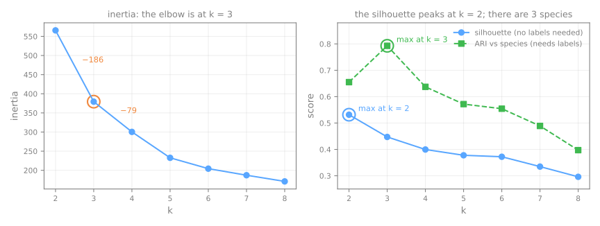
Leia a tabela como num projeto real, tapando a última coluna. A inércia cai 186,3 de \(k=2\) para 3 e depois só 79,0 de 3 para 4: um cotovelo em 3. A silhueta, o Calinski–Harabasz e o Davies–Bouldin preferem, os três, \(k = 2\) (0,532; 482,2 e 0,714). Agora destape o ARI: ele é máximo em \(k = 3\), 0,793, as três espécies. Os índices internos não erraram sobre o que medem. Os pinguins Adélia e de barbicha têm quase a mesma massa e as mesmas nadadeiras e diferem principalmente no comprimento do bico, então juntá-los dá uma partição que é de fato mais coesa e mais separada. "Quão separada é esta partição" e "esta é a partição que eu quero" são perguntas diferentes; nenhum índice interno responde à segunda. Aqui o cotovelo por acaso acertou; isso é sorte deste conjunto de dados, não regra.
Varra o \(k\) nos oito conjuntos do simulador. Em bolhas limpas, o cotovelo e a silhueta concordam; em tamanhos desiguais, a silhueta aponta 2; em círculos e grupos alongados, ela não tem máximo interior; e no ruído ela ainda devolve um número para cada \(k\):
Esse último caso merece um número. Ruído uniforme não tem grupo nenhum:
R = np.random.default_rng(0).random((300, 2))                    # 300 pontos uniformes: nenhuma estrutura
for k in range(2, 6):
    lab = KMeans(n_clusters=k, n_init=10, random_state=0).fit_predict(R)
    print(k, round(silhouette_score(R, lab), 3))
Uma silhueta de 0,40 tirada de puro ruído, na mesma faixa dos pinguins. A silhueta, portanto, não é um atestado de que existem grupos. Uma régua útil é rodar o mesmo pipeline nos seus dados com cada coluna embaralhada de forma independente (o que preserva a distribuição de cada coluna e destrói as relações entre elas) e relatar a silhueta real ao lado da embaralhada; o lab faz exatamente isso.
A escala importa (e a silhueta não vai avisar)
Os mesmos pinguins, agrupados nas unidades originais e padronizados:
print(peng[num].std().round(2).to_dict())
for name, M in [('raw units', peng[num].to_numpy()), ('standardized', Z)]:
    lab = KMeans(n_clusters=3, n_init=10, random_state=0).fit_predict(M)
    print(f"{name:13s} silhouette {silhouette_score(M, lab):.3f}   ARI with species {adjusted_rand_score(species, lab):.3f}")
{'culmen_length_mm': 5.46, 'culmen_depth_mm': 1.97, 'flipper_length_mm': 14.06, 'body_mass_g': 801.95}
raw units     silhouette 0.580   ARI with species 0.331
standardized  silhouette 0.447   ARI with species 0.793
O desvio padrão da massa corporal é cerca de 400 vezes o da profundidade do bico, então a distância euclidiana bruta é essencialmente uma diferença em gramas: o k-means separa os pinguins em três faixas de peso. Essas faixas são bem separadas e a silhueta prefere os dados brutos (0,580 contra 0,447). As espécies são recuperadas muito melhor depois de padronizar (ARI 0,793 contra 0,331). Sem rótulos, que é a situação real, seguir a silhueta teria levado você ao pré-processamento errado. Um índice interno compara partições do mesmo espaço; quando a escala muda, a régua muda junto. Escalonar ou não se decide por um argumento sobre as unidades (um grama e um milímetro não são comparáveis), não por um índice. Padronizar é a escolha usual; a aula de Pré-processamento compara os escalonadores.
O que o k-means supõe e onde ele falha
Etapa 4. Cada grupo do k-means é o conjunto dos pontos mais próximos de um centro do que de qualquer outro: uma célula convexa de um diagrama de Voronoi, separada das vizinhas por fronteiras retas a meio caminho entre os centros. E a inércia cobra de cada ponto o mesmo quadrado da distância, seja qual for o seu grupo. Isso embute suposições:
- os grupos são convexos e mais ou menos redondos (isotrópicos): nada de luas crescentes, anéis ou faixas diagonais compridas;
- os grupos têm espalhamento parecido: um grupo largo perde os seus pontos de fora para um vizinho compacto;
- não há ruído: todo ponto vai para algum grupo, outliers incluídos;
- você sabe o \(k\).
Cinco conjuntos 2-D de 500 pontos cujos grupos verdadeiros são conhecidos; o k-means recebe o \(k\) correto:
from sklearn.datasets import make_circles, make_moons

Xa, ya = make_blobs(n_samples=500, centers=3, random_state=170)
shapes = {
    'blobs':       make_blobs(n_samples=500, centers=3, cluster_std=1.0, random_state=8),
    'moons':       make_moons(n_samples=500, noise=0.06, random_state=0),
    'circles':     make_circles(n_samples=500, factor=0.5, noise=0.05, random_state=0),
    'anisotropic': (Xa @ np.array([[0.6, -0.6], [-0.4, 0.8]]), ya),    # bolhas esticadas
    'densities':   make_blobs(n_samples=[150, 150, 200], centers=[[0, 0], [1.2, 0], [4, 2]],
                              cluster_std=[0.2, 0.2, 1.0], random_state=0),
}
for name, (Xs, ys) in shapes.items():
    k = len(np.unique(ys))
    lab = KMeans(n_clusters=k, n_init=10, random_state=0).fit_predict(Xs)
    print(f"{name:12s} k={k}  silhouette {silhouette_score(Xs, lab):.3f}   ARI {adjusted_rand_score(ys, lab):6.3f}")
blobs        k=3  silhouette 0.823   ARI  1.000
moons        k=2  silhouette 0.489   ARI  0.253
circles      k=2  silhouette 0.356   ARI -0.002
anisotropic  k=3  silhouette 0.501   ARI  0.555
densities    k=3  silhouette 0.605   ARI  0.436
Só as bolhas (blobs) são recuperadas. As luas (moons) são cortadas de través (ARI 0,253), os círculos concêntricos (circles) são divididos em dois semidiscos, o que é exatamente tão bom quanto o acaso (ARI −0,002); os grupos esticados (anisotropic) são divididos na diagonal errada (0,555). Em densities, dois grupos compactos ficam lado a lado junto de um largo: o k-means junta os dois compactos e corta o largo em dois (0,436), porque isso baixa mais a inércia do que respeitar os grupos verdadeiros. Agora leia a coluna da silhueta: ela não ordena os agrupamentos pelo acerto. Densities, em que o k-means errou os três grupos (ARI 0,436), tem a segunda maior silhueta, 0,605, acima dos agrupamentos esticado e das luas. A métrica não avisa, porque compartilha a ideia de bom grupo do algoritmo: compacto e longe dos outros. Percorra os formatos e varie o \(k\) aqui; nenhum valor de \(k\) conserta um anel:
Agrupamento hierárquico
O k-means devolve uma partição plana para um \(k\) escolhido; o agrupamento hierárquico (aglomerativo), em vez disso, constrói a árvore inteira de fusões sucessivas (o dendrograma) e deixa você escolher o número de grupos depois, cortando-a. Ele tem a sua própria aula, Agrupamento Hierárquico, em que as ligações (single, complete, average, Ward) são calculadas à mão.
DBSCAN e HDBSCAN: agrupamento por densidade
O DBSCAN (Ester et al., 1996) parte de outra ideia de grupo: uma região densa, separada das outras regiões densas por regiões esparsas. Ele tem dois parâmetros (um raio eps e uma contagem min_samples) e classifica os pontos em três tipos:
- ponto central (core): tem pelo menos
min_samplespontos a uma distância de atéeps, contando ele mesmo (a convenção do scikit-learn); - ponto de borda (border): não é central, mas está a até
epsde um ponto central; - ruído (noise): nenhum dos dois. O ruído recebe o rótulo −1: o DBSCAN não força outliers para dentro de um grupo.
Um grupo é então um conjunto de pontos centrais que se alcançam uns aos outros por saltos de comprimento até eps passando por pontos centrais, mais os pontos de borda ligados a eles. Os grupos podem ter qualquer forma e ninguém escolhe quantos são.
DBSCAN, à mão
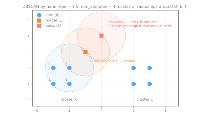
Dez pontos, eps = 1.5, min_samples = 4. \(A, B, C, D\) formam um quadrado de lado 1 embaixo à esquerda; \(E = (3, 3)\) e \(F = (4, 4)\) se afastam dele na diagonal; \(G, H, I, J\) formam outro quadrado de lado 1 embaixo à direita. Conte, para cada ponto, os pontos a até 1,5 (ele incluído); num quadrado de lado 1, os outros vértices estão a 1, 1 e 1,414:
| ponto | coordenadas | pontos a até 1,5 (ele incluído) | central? | alcança um central? | tipo |
|---|---|---|---|---|---|
| A, B, C, D | o quadrado da esquerda | 4 (o quadrado), +1 para D, que também vê E | sim | central | |
| E | (3, 3) | 3: E, D (1,414), F (1,414) | não | sim, D | borda |
| F | (4, 4) | 2: F, E (1,414) | não | não, E não é central | ruído |
| G, H, I, J | o quadrado da direita | 4 | sim | central |
\(F\) é o caso instrutivo: está a até eps de \(E\), que pertence a um grupo, mas \(E\) é só um ponto de borda; os grupos só crescem através de pontos centrais. Então \(F\) é ruído.
from sklearn.cluster import DBSCAN

P = np.array([[1, 1], [2, 1], [1, 2], [2, 2], [3, 3], [4, 4], [6, 1], [7, 1], [6, 2], [7, 2]], dtype=float)
names = list('ABCDEFGHIJ')
DP = np.sqrt(((P[:, None, :] - P[None, :, :]) ** 2).sum(axis=2))
print('within eps:', dict(zip(names, (DP <= 1.5).sum(axis=1).tolist())))   # ele mesmo incluído
db = DBSCAN(eps=1.5, min_samples=4).fit(P)
print('core:  ', [names[i] for i in db.core_sample_indices_])
print('labels:', dict(zip(names, db.labels_.tolist())))
within eps: {'A': 4, 'B': 4, 'C': 4, 'D': 5, 'E': 3, 'F': 2, 'G': 4, 'H': 4, 'I': 4, 'J': 4}
core:   ['A', 'B', 'C', 'D', 'G', 'H', 'I', 'J']
labels: {'A': 0, 'B': 0, 'C': 0, 'D': 0, 'E': 0, 'F': -1, 'G': 1, 'H': 1, 'I': 1, 'J': 1}
As contagens batem com a tabela, os pontos centrais são os oito vértices dos dois quadrados, \(E\) entra no grupo 0 como ponto de borda e \(F\) recebe −1.
Escolhendo o eps: o gráfico de k-distâncias
eps é uma distância; um bom valor depende inteiramente da escala e da densidade dos dados. A ferramenta padrão (proposta no próprio artigo do DBSCAN) é o gráfico de k-distâncias: para cada ponto, a distância ao seu \(k\)-ésimo vizinho mais próximo, com \(k\) = min_samples (de novo contando o próprio ponto), em ordem crescente. Um ponto é central exatamente quando essa distância é no máximo eps. Dentro de uma região densa a distância é pequena; a curva dobra bruscamente para cima onde começam os pontos esparsos; o eps é lido nesse joelho.
Isso funciona quando há uma densidade só. Tome de novo os dados densities: dois grupos compactos (desvio padrão 0,2) e um grupo frouxo (1,0).
from sklearn.neighbors import NearestNeighbors

X_dens, y_dens = shapes['densities']
kdist = NearestNeighbors(n_neighbors=5).fit(X_dens).kneighbors(X_dens)[0][:, -1]   # 5º vizinho, ele mesmo incluído
for g in range(3):
    print(f"group {g}: median distance to the 5th neighbor {np.median(kdist[y_dens == g]):.3f}")
for eps in [0.1, 0.15, 0.2, 0.3, 0.4, 0.6, 0.8]:
    lab = DBSCAN(eps=eps, min_samples=5).fit_predict(X_dens)
    print(f"eps {eps:<4}: {lab.max() + 1} clusters (largest {np.bincount(lab[lab >= 0]).max()}), "
          f"{(lab == -1).sum():3d} noise, ARI {adjusted_rand_score(y_dens, lab):6.3f}")
group 0: median distance to the 5th neighbor 0.070
group 1: median distance to the 5th neighbor 0.065
group 2: median distance to the 5th neighbor 0.293
eps 0.1 : 5 clusters (largest 134), 225 noise, ARI  0.740
eps 0.15: 8 clusters (largest 146), 172 noise, ARI  0.825
eps 0.2 : 9 clusters (largest 149), 137 noise, ARI  0.789
eps 0.3 : 6 clusters (largest 300),  63 noise, ARI  0.397
eps 0.4 : 2 clusters (largest 300),  28 noise, ARI  0.556
eps 0.6 : 2 clusters (largest 301),   5 noise, ARI  0.619
eps 0.8 : 1 clusters (largest 496),   4 noise, ARI -0.003
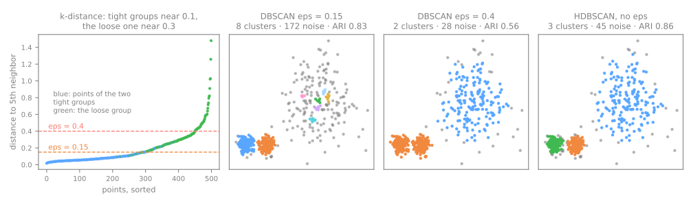
Os grupos compactos pedem um eps de cerca de 0,07; o frouxo, de cerca de 0,3, quatro vezes mais. Todo valor único falha em algum lugar. Até eps = 0.2 os dois grupos compactos são encontrados (nenhum grupo passa de 149 pontos, então os dois ficam separados), enquanto o frouxo se estilhaça em fragmentos e ruído: 172 pontos de ruído em 0,15. Em eps = 0.3 os dois compactos já se fundiram num grupo de 300 pontos, enquanto o frouxo ainda está em pedaços; em 0,4 e 0,6 há dois grupos, o par fundido e o grupo frouxo; em 0,8, tudo é um grupo só. Em nenhum ponto da varredura aparecem os três grupos. Um eps global significa uma densidade: essa é a limitação central do DBSCAN.
HDBSCAN: todos os valores de eps de uma vez
O HDBSCAN (Campello, Moulavi & Sander, 2013) elimina o eps. Informalmente, ele roda o DBSCAN para todos os eps possíveis de uma vez: conforme o eps diminui, os grupos se dividem, perdem pontos para o ruído ou desaparecem; o resultado é uma hierarquia de grupos. O HDBSCAN então fica com os grupos que persistem na faixa mais larga de densidades (os mais estáveis), cada um no seu próprio nível de densidade. Um grupo compacto e um frouxo podem ser mantidos os dois, porque não precisam existir no mesmo eps. O principal parâmetro que sobra é min_cluster_size, o menor grupo que você aceita chamar de grupo, sobre o qual é muito mais fácil raciocinar do que sobre uma distância.
from sklearn.cluster import HDBSCAN

for name, (Xs, ys) in shapes.items():
    lab = HDBSCAN(min_cluster_size=15).fit_predict(Xs)
    print(f"{name:12s} {lab.max() + 1} clusters, {(lab == -1).sum():2d} noise, ARI {adjusted_rand_score(ys, lab):.3f}")
blobs        3 clusters,  0 noise, ARI 1.000
moons        2 clusters,  0 noise, ARI 1.000
circles      2 clusters,  0 noise, ARI 1.000
anisotropic  3 clusters, 49 noise, ARI 0.852
densities    3 clusters, 45 noise, ARI 0.856
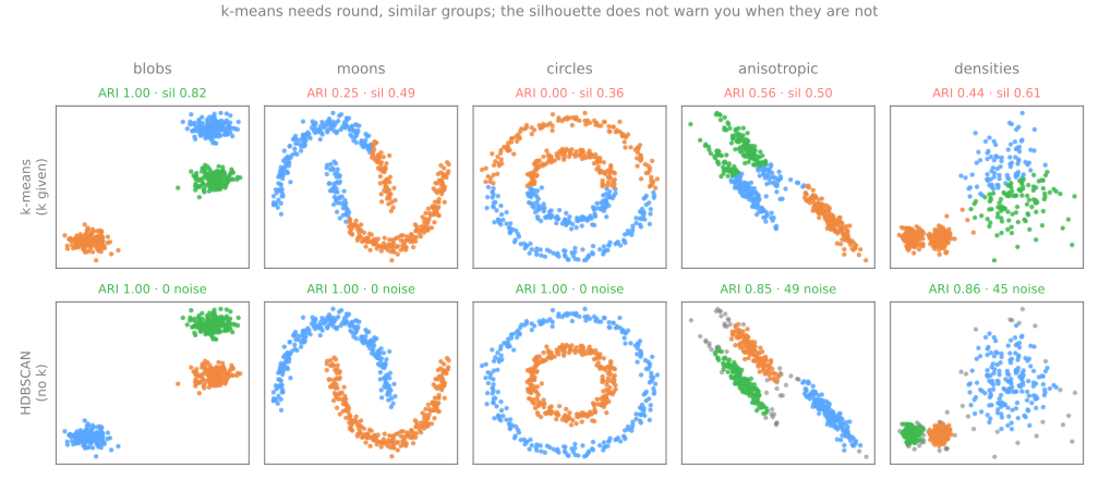
Sem ser informado do \(k\), o HDBSCAN encontra o número certo de grupos nos cinco conjuntos e recupera as luas e os anéis exatamente. Nos grupos esticados e em densities, ele rotula como ruído 49 e 45 pontos (as caudas finas e a franja do grupo frouxo). O ARI conta ruído como erro, daí 0,852 e 0,856; os pontos que ele atribuiu estão todos no grupo certo. Se chamar pontos da franja de "ruído" é defeito ou virtude depende da aplicação. É o motivo pelo qual o BERTopic usa o HDBSCAN sobre embeddings de documentos: documentos que não se encaixam em tópico nenhum viram ruído em vez de poluir um tópico.
O HDBSCAN não está livre de suposições. min_cluster_size ainda importa: nos círculos, subi-lo para 30 transforma todos os pontos em ruído. E todo método de densidade sofre em muitas dimensões, onde cada ponto fica mais ou menos igualmente longe de todos os outros e "denso" perde o sentido: o lab mede isso nas 13 medidas dos vinhos.
Escolhendo um algoritmo
| k-means | hierárquico (Ward) | DBSCAN | HDBSCAN | |
|---|---|---|---|---|
| um grupo é | os pontos mais próximos de um centro | o que se funde primeiro numa árvore de fusões | uma região densa | uma região densa, na sua própria densidade |
| você escolhe | \(k\) | onde cortar a árvore (\(k\)) | eps, min_samples | min_cluster_size |
| formas | convexas, redondas, espalhamento parecido | depende da ligação | quaisquer | quaisquer, com densidades diferentes |
| ruído / outliers | forçados para um grupo | forçados para um grupo | rotulados −1 | rotulados −1 |
| pontos novos | predict para o centro mais próximo | sem predict | sem predict | sem predict |
| escala até | milhões de linhas (MiniBatchKMeans) | milhares (memória quadrática) | \(n\) grande, poucas dimensões | \(n\) grande, poucas dimensões |
Etapa 5. Comece pelo k-means: é rápido, o seu critério (a inércia) e a sua nota usual (a silhueta) são bem entendidos e ele sabe atribuir pontos novos. Troque quando tiver um motivo concreto: grupos visivelmente não convexos, densidades muito diferentes, outliers que não podem ser forçados para um grupo ou nenhuma forma de justificar um \(k\). Os modelos de mistura de gaussianas (GaussianMixture) são o outro passo comum além do k-means: cada grupo ganha a sua própria forma elíptica e cada ponto, uma probabilidade de pertencer a ele; um dos exercícios de extensão do lab os experimenta.
Quatro perguntas antes de acreditar num agrupamento
- Padronizei? Se não, o agrupamento provavelmente está ordenando pela coluna de maior unidade.
- Reiniciei o suficiente?
n_initbem acima de 1; do contrário, uma inércia dez vezes maior que a melhor é possível. - De onde veio o \(k\)? Se veio só da silhueta, lembre-se de que ela preferiu 2 grupos de pinguins onde há 3 espécies.
- Comparei com dados embaralhados? Ruído puro chega a uma silhueta de 0,40.
Interpretando os grupos
Uma partição só é útil se alguém consegue dizer o que cada grupo é. Centros em unidades padronizadas não se leem, então volte às colunas originais e descreva cada grupo com um groupby, exatamente como na AED:
peng['cluster'] = KMeans(n_clusters=3, n_init=10, random_state=0).fit_predict(Z)
print(peng.groupby('cluster')[num].mean().round(1).assign(n=peng['cluster'].value_counts()))
print(pd.crosstab(peng['cluster'], species))                    # uma conferência que só aqui podemos fazer
         culmen_length_mm  culmen_depth_mm  flipper_length_mm  body_mass_g    n
cluster
0                    47.5             15.0              217.2       5076.0  123
1                    38.2             18.1              188.4       3584.7  132
2                    47.5             18.8              196.9       3902.0   87
species  Adelie  Chinstrap  Gentoo
cluster
0             0          0     123
1           127          5       0
2            24         63       0
O perfil é uma descrição que qualquer um confere: um grupo de aves pesadas, de nadadeiras longas e bico raso; um de bicos longos e profundos; um de aves pequenas de bico curto. É o que você escreveria num relatório sem rótulos. A tabela cruzada é o luxo deste conjunto de dados: o primeiro grupo é exatamente o dos pinguins-gentoo; a única confusão é entre Adélia e de barbicha, as duas espécies que diferem principalmente no comprimento do bico, justamente o par que a silhueta queria juntar.
Ao relatar o resultado, descreva uma escolha, não uma descoberta. Não "encontramos 3 segmentos", mas "particionamos os dados em 3 grupos depois de padronizar, escolhemos \(k\) por tal critério e o resultado está a tal distância do que dados embaralhados dão". A diferença não é de estilo: a primeira frase afirma algo sobre o mundo, a segunda declara uma decisão, o seu critério e a evidência de que o resultado não é ruído. O final do lab escreve um parágrafo assim, com números reais.
Exercícios
- Refaça a conta à mão do algoritmo de Lloyd com o começo bom \(c_1 = (1, 1)\), \(c_2 = (7, 6)\). Quantas iterações ele leva? Qual é a inércia depois da primeira atribuição?
- Para os oito pontos, calcule \(s(x_4)\) à mão e confira com
silhouette_samples. Depois mova \(x_4\) para \((3, 3)\), recalcule a silhueta dele e explique a mudança usando \(a\) e \(b\). - No exemplo do DBSCAN, qual é o menor
epspara o qual \(F\) deixa de ser ruído commin_samples = 4? E o menor para o qual os dois quadrados se fundem num grupo só? Confira com o scikit-learn. - Construa 300 pontos em que um atributo é uniforme em \([0, 1]\) e outro em \([0, 1000]\), com três grupos verdadeiros separados só ao longo do primeiro atributo. Compare o ARI do k-means com e sem padronização.
Lab: agrupar 178 vinhos
O conjunto de dados é o usado no roteiro de laboratório do professor: 178 vinhos italianos de três cultivares, cada um descrito por 13 medidas químicas, embutido no scikit-learn. A regra do lab: a coluna da cultivar fica lacrada até o último passo. Toda decisão (escala, \(k\), algoritmo) tem de ser tomada com as ferramentas que existem quando não há rótulos; só no fim abrimos o gabarito, para auditar essas decisões. Num projeto real, esse último passo não existe.
Rode os blocos em ordem, numa mesma sessão. Toda saída abaixo é o que o código imprime. Para trabalhar direto nele, baixe o notebook do lab e abra no Jupyter ou no Colab (Arquivo → Fazer upload de notebook); ele só precisa de scikit-learn, pandas, numpy e matplotlib.
Passo 1 — carregar e lacrar a cultivar
import numpy as np
import pandas as pd
import matplotlib.pyplot as plt
from sklearn.datasets import load_wine

wine = load_wine(as_frame=True)
df = wine.frame
cultivar = df.pop('target')                 # a cultivar verdadeira: lacrada até o passo 9
print(df.shape, '· missing values:', int(df.isna().sum().sum()))
sd = df.std().sort_values()
print(sd.iloc[[0, 1, -2, -1]].round(3))
print(f"largest std / smallest std = {sd.iloc[-1] / sd.iloc[0]:.0f}")
(178, 13) · missing values: 0
nonflavanoid_phenols      0.124
hue                       0.229
magnesium                14.282
proline                 314.907
dtype: float64
largest std / smallest std = 2530
Como ler: 178 vinhos, 13 colunas numéricas, nada faltando. As colunas estão em escalas muito diferentes: a prolina tem desvio padrão de 314,9, os fenóis não flavonoides 0,124, uma razão de 2.530. Nas unidades originais, qualquer distância euclidiana entre dois vinhos é essencialmente a diferença de prolina entre eles.
Passo 2 — escalonar e por que os índices não podem decidir isso
from sklearn.cluster import KMeans
from sklearn.metrics import calinski_harabasz_score, davies_bouldin_score, silhouette_score
from sklearn.preprocessing import MinMaxScaler, RobustScaler, StandardScaler

X = df.to_numpy()
scalers = {'none': None, 'StandardScaler': StandardScaler(), 'MinMaxScaler': MinMaxScaler(),
           'RobustScaler': RobustScaler()}
for name, scaler in scalers.items():
    M = X if scaler is None else scaler.fit_transform(X)
    lab = KMeans(n_clusters=3, n_init=10, random_state=0).fit_predict(M)
    print(f"{name:15s} silhouette {silhouette_score(M, lab):.3f}   CH {calinski_harabasz_score(M, lab):6.1f}"
          f"   DB {davies_bouldin_score(M, lab):.3f}")

Z = StandardScaler().fit_transform(X)       # a escolha, feita por argumento
none            silhouette 0.571   CH  561.8   DB 0.534
StandardScaler  silhouette 0.285   CH   70.9   DB 1.389
MinMaxScaler    silhouette 0.301   CH   83.4   DB 1.305
RobustScaler    silhouette 0.264   CH   61.1   DB 1.466
Como ler: os três índices internos são unânimes em preferir não escalonar: silhueta 0,571 contra 0,285, um Calinski–Harabasz oito vezes maior, um Davies–Bouldin (quanto menor, melhor) 2,6 vezes menor. Sem escalonar, o espaço é essencialmente o eixo da prolina, cujas faixas são muito bem separadas. Como nos pinguins, os índices medem separação no espaço que você lhes dá, então compará-los entre escalas compara réguas, não partições. Padronizamos mesmo assim, porque uma distância que soma porcentagem de álcool com miligramas de prolina por litro e razões de absorbância não tem sentido; o passo 9 dirá se isso estava certo.
Passo 3 — escolher k com o cotovelo e a silhueta
rows = []
for k in range(2, 9):
    m = KMeans(n_clusters=k, n_init=10, random_state=0).fit(Z)
    rows.append({'k': k, 'inertia': m.inertia_, 'silhouette': silhouette_score(Z, m.labels_),
                 'CH': calinski_harabasz_score(Z, m.labels_), 'DB': davies_bouldin_score(Z, m.labels_)})
scores = pd.DataFrame(rows).set_index('k')
print(scores.round(3))

fig, (ax1, ax2) = plt.subplots(1, 2, figsize=(9, 3.2))
scores['inertia'].plot(ax=ax1, marker='o', title='inércia: procure o cotovelo')
scores['silhouette'].plot(ax=ax2, marker='o', title='silhueta: quanto maior, melhor')
plt.tight_layout()
plt.show()
    inertia  silhouette      CH     DB
k
2  1659.008       0.268  69.486  1.448
3  1277.928       0.285  70.940  1.389
4  1180.738       0.246  55.668  1.765
5  1110.365       0.203  46.883  1.820
6  1044.470       0.196  41.812  1.812
7   995.995       0.139  37.714  1.922
8   944.559       0.158  35.210  1.769
Como ler: a inércia cai 381,1 de \(k = 2\) para 3 e só 97,2 de 3 para 4, um cotovelo em 3. A silhueta, o Calinski–Harabasz e o Davies–Bouldin também apontam \(k = 3\). Mas olhe a margem: a silhueta separa \(k = 3\) (0,285) de \(k = 2\) (0,268) por apenas 0,017, o tipo de diferença que uma amostra um pouco diferente apagaria. O primeiro exercício de extensão mede um critério que separa os dois com muito mais clareza.
Passo 4 — a régua: o mesmo pipeline em dados embaralhados
rng = np.random.default_rng(0)
Z_shuffled = Z.copy()
for j in range(Z_shuffled.shape[1]):
    rng.shuffle(Z_shuffled[:, j])           # destrói a relação entre colunas, preserva cada coluna
for k in [2, 3, 4]:
    lab = KMeans(n_clusters=k, n_init=10, random_state=0).fit_predict(Z_shuffled)
    print(k, round(silhouette_score(Z_shuffled, lab), 3), round(calinski_harabasz_score(Z_shuffled, lab), 1))
Como ler: embaralhar cada coluna de forma independente preserva a distribuição de cada medida, mas destrói qualquer estrutura que esteja na combinação das colunas. Nesses vinhos sem estrutura, o k-means com \(k = 3\) chega a uma silhueta de 0,068 e um Calinski–Harabasz de 13,3. Os dados reais dão 0,285 e 70,9: cerca de quatro e cinco vezes mais. Uma silhueta de 0,285 parece baixa em termos absolutos (os oito pontos deram 0,82); sem essa régua, você poderia ter descartado o agrupamento. Com ela, dá para dizer que os grupos são muito mais separados do que qualquer coisa que dados embaralhados produzem.
Passo 5 — ajustar k = 3 e inspecionar cada grupo
from sklearn.metrics import silhouette_samples

km = KMeans(n_clusters=3, n_init=10, random_state=0).fit(Z)
labels = km.labels_
s = silhouette_samples(Z, labels)
for j in range(3):
    print(f"cluster {j}: {np.sum(labels == j):3d} wines · mean silhouette {s[labels == j].mean():.3f}"
          f" · negative silhouettes {np.sum(s[labels == j] < 0)}")
cluster 0:  65 wines · mean silhouette 0.177 · negative silhouettes 7
cluster 1:  51 wines · mean silhouette 0.351 · negative silhouettes 0
cluster 2:  62 wines · mean silhouette 0.343 · negative silhouettes 0
Como ler: a silhueta média de 0,285 esconde dois tipos de grupo. Os grupos 1 e 2 (51 e 62 vinhos) têm silhuetas perto de 0,35 e nenhum ponto negativo. O grupo 0 (65 vinhos) tem metade dessa coesão (0,177) e 7 vinhos mais perto, em média, de outro grupo do que do próprio. Mantenha a hipótese em aberto: o grupo 0 é mal formado ou só espalhado? O passo 9 responde.
Passo 6 — o perfil dos grupos nas unidades originais
cols = ['alcohol', 'flavanoids', 'color_intensity', 'proline', 'od280/od315_of_diluted_wines']
print(df.assign(cluster=labels).groupby('cluster')[cols].mean().round(2).to_string())

z_means = pd.DataFrame(Z, columns=df.columns).assign(cluster=labels).groupby('cluster').mean()
for j, row in z_means.iterrows():
    top = row[row.abs().sort_values(ascending=False).index[:3]]
    print(f"cluster {j}:", ', '.join(f"{c} {v:+.2f} sd" for c, v in top.items()))
         alcohol  flavanoids  color_intensity  proline  od280/od315_of_diluted_wines
cluster
0          12.25        2.05             2.97   510.17                          2.80
1          13.13        0.82             7.23   619.06                          1.70
2          13.68        3.00             5.45  1100.23                          3.16
cluster 0: alcohol -0.93 sd, color_intensity -0.90 sd, proline -0.75 sd
cluster 1: od280/od315_of_diluted_wines -1.29 sd, flavanoids -1.22 sd, hue -1.16 sd
cluster 2: proline +1.13 sd, flavanoids +0.98 sd, total_phenols +0.89 sd
Como ler: a primeira tabela é um groupby de AED nas unidades originais, que um enólogo consegue ler. A segunda lista, para cada grupo, as três medidas em que a sua média está mais longe da média geral, em desvios padrão. Agora os grupos podem receber nomes. O grupo 2 é rico em prolina (1.100 em média, contra 510 e 619), flavonoides e fenóis; é também o mais alcoólico (13,68%). O grupo 1 tem poucos flavonoides (0,82), OD280 baixo (uma medida do conteúdo fenólico), matiz baixo e a cor mais intensa (7,23). O grupo 0 é o leve: 0,93 desvio padrão abaixo da média em álcool, 0,90 em intensidade de cor, 0,75 em prolina. Um agrupamento que ninguém consegue descrever assim raramente é útil, por melhor que seja a sua silhueta.
Passo 7 — experimentar o DBSCAN e o HDBSCAN
from sklearn.cluster import DBSCAN, HDBSCAN
from sklearn.neighbors import NearestNeighbors

kdist = NearestNeighbors(n_neighbors=5).fit(Z).kneighbors(Z)[0][:, -1]
print('distance to the 5th neighbor, percentiles 10/50/90:', np.percentile(kdist, [10, 50, 90]).round(2))
for eps in [1.8, 2.0, 2.2, 2.4, 2.6]:
    lab = DBSCAN(eps=eps, min_samples=5).fit_predict(Z)
    print(f"DBSCAN eps {eps}: {lab.max() + 1} clusters, {np.sum(lab == -1):3d} noise")
hd = HDBSCAN(min_cluster_size=10).fit_predict(Z)
print(f"HDBSCAN min_cluster_size=10: {hd.max() + 1} clusters, {np.sum(hd == -1)} noise")
distance to the 5th neighbor, percentiles 10/50/90: [1.83 2.22 3.13]
DBSCAN eps 1.8: 7 clusters, 118 noise
DBSCAN eps 2.0: 5 clusters,  85 noise
DBSCAN eps 2.2: 2 clusters,  55 noise
DBSCAN eps 2.4: 2 clusters,  36 noise
DBSCAN eps 2.6: 1 clusters,  20 noise
HDBSCAN min_cluster_size=10: 2 clusters, 75 noise
Como ler: em 13 dimensões padronizadas, a distância de um vinho ao seu 5º vizinho vai só de 1,83 a 3,13 entre os percentis 10 e 90. Não há região claramente mais densa que o resto, o que é típico em muitas dimensões, onde todos os pontos tendem a ficar mais ou menos igualmente distantes (a maldição da dimensionalidade). O DBSCAN reflete isso. Um eps pequeno deixa a maioria dos vinhos como ruído e quebra o resto em fragmentos (7 grupos e 118 pontos de ruído em 1,8); um grande junta tudo num grupo só (2,6); entre os dois, ele encontra dois grupos, com 36 a 55 pontos de ruído. Nunca encontra três. O HDBSCAN encontra 2 grupos e chama 75 dos 178 vinhos de ruído. Métodos de densidade são a ferramenta certa para formas arbitrárias em poucas dimensões; aqui, a suposição de grupos redondos do k-means se encaixa melhor, como o último passo vai confirmar.
Passo 8 — olhar os grupos com a PCA
from sklearn.decomposition import PCA

pca = PCA(n_components=2).fit(Z)
A = pca.transform(Z)
print('variance kept by 2 components:', pca.explained_variance_ratio_.round(3),
      round(pca.explained_variance_ratio_.sum(), 3))

lab_2d = KMeans(n_clusters=3, n_init=10, random_state=0).fit_predict(A)
print('k-means on the 2 components, silhouette measured in 2-D :', round(silhouette_score(A, lab_2d), 3))
print('the same partition, silhouette measured in 13-D         :', round(silhouette_score(Z, lab_2d), 3))

fig, (ax1, ax2) = plt.subplots(1, 2, figsize=(10, 4), sharex=True, sharey=True)
ax1.scatter(A[:, 0], A[:, 1], c=labels, cmap='tab10', vmin=0, vmax=9, s=15)
ax1.set_title('k-means, k = 3 (ajustado em 13-D)')
ax2.scatter(A[:, 0], A[:, 1], c=np.where(hd == -1, 7, hd), cmap='tab10', vmin=0, vmax=9, s=15)
ax2.set_title('HDBSCAN (cinza = ruído)')
plt.show()
variance kept by 2 components: [0.362 0.192] 0.554
k-means on the 2 components, silhouette measured in 2-D : 0.561
the same partition, silhouette measured in 13-D         : 0.283
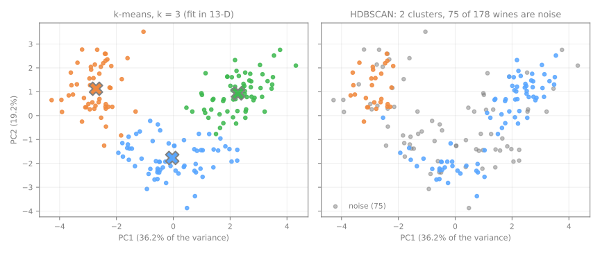
Como ler: as duas primeiras componentes principais (Redução de Dimensionalidade) guardam 55,4% da variância, o bastante para ver os três grupos do k-means como três regiões do plano, com o ruído do HDBSCAN espalhado por todas elas. O plano é uma janela, não o espaço onde o agrupamento aconteceu. Agrupar no plano muda pouco: a partição encontrada nas 2 componentes tem silhueta de 0,283 quando medida no espaço completo de 13 dimensões, praticamente a mesma de antes. Mas medida em 2-D, a mesma partição marca 0,561, o dobro. Não é um agrupamento melhor, é uma régua mais curta: em 2-D a silhueta ignora as 11 direções em que os grupos se sobrepõem. Reduza para visualizar (ou para acelerar), se quiser, mas meça no espaço em que você faz a afirmação.
Passo 9 — abrir o lacre: auditar cada decisão
from sklearn.metrics import adjusted_rand_score

partitions = {
    'k-means k=3, standardized': labels,
    'k-means k=2, standardized': KMeans(n_clusters=2, n_init=10, random_state=0).fit_predict(Z),
    'k-means k=3, raw units':    KMeans(n_clusters=3, n_init=10, random_state=0).fit_predict(X),
    'k-means k=3, on 2 PCs':     lab_2d,
    'DBSCAN eps=2.4':            DBSCAN(eps=2.4, min_samples=5).fit_predict(Z),
    'HDBSCAN':                   hd,
}
for name, lab in partitions.items():
    print(f"{name:27s} ARI {adjusted_rand_score(cultivar, lab):.3f}")
print(pd.crosstab(labels, cultivar, rownames=['cluster'], colnames=['cultivar']))
k-means k=3, standardized   ARI 0.897
k-means k=2, standardized   ARI 0.389
k-means k=3, raw units      ARI 0.371
k-means k=3, on 2 PCs       ARI 0.895
DBSCAN eps=2.4              ARI 0.421
HDBSCAN                     ARI 0.263
cultivar   0   1   2
cluster
0          0  65   0
1          0   3  48
2         59   3   0
Como ler: o gabarito audita cada decisão.
- A escala. Sem escalonar, o k-means recupera as cultivares com ARI de 0,371; padronizado, 0,897. Os três índices internos do passo 2 foram unânimes a favor da resposta errada. Nenhum índice geométrico poderia ter salvado essa decisão; ela se apoia no argumento sobre as unidades.
- O \(k\). \(k = 2\) teria dado 0,389, contra 0,897 de \(k = 3\). A silhueta escolheu certo, mas por uma margem de 0,017.
- O grupo 0. Ele tinha a pior silhueta (0,177) e 7 valores negativos, mas a tabela cruzada mostra que ele é 100% puro: os seus 65 vinhos são todos da cultivar 1. Silhueta baixa significa grupo espalhado, não grupo errado. Os 6 erros do k-means (172 de 178 vinhos certos) estão nos grupos 1 e 2, os de silhueta alta.
- O algoritmo. O DBSCAN (0,421) e o HDBSCAN (0,263) ficam muito atrás: em 13 dimensões não há vales de densidade claros para seguir.
- A PCA. Agrupar nas 2 componentes quase não perde nada (0,895), o que o passo 8 já sugeria; o que enganava era a sua silhueta de 0,561.
Num projeto real este passo não existe: tudo acima teria sido decidido com os passos 1 a 8. O parágrafo que você escreveria seria então algo como: "As 13 medidas foram padronizadas, já que as suas escalas diferem por um fator de até 2.530. Os vinhos foram particionados com k-means (n_init=10); \(k = 3\) foi escolhido porque o cotovelo da inércia e os três índices internos concordam nele, embora a silhueta separe \(k = 3\) de \(k = 2\) por apenas 0,017. A silhueta, 0,285, se compara a 0,068 nos mesmos dados com as colunas embaralhadas. Um dos três grupos é bem menos coeso (silhueta média 0,177, 7 vinhos com silhueta negativa) e deve ser interpretado com cautela." Ele declara o pré-processamento e o motivo, o critério para \(k\) e a sua fraqueza, a linha de base e a fragilidade conhecida; em nenhum momento afirma ter "descoberto" três tipos de vinho.
Sua vez
- Estabilidade. Um grupo real deveria reaparecer quando os dados são reamostrados. Para \(k = 2, \dots, 7\), agrupe 30 subamostras aleatórias com 80% dos vinhos e, para cada par de subamostras, calcule o ARI entre os rótulos dos vinhos que elas têm em comum. Qual \(k\) dá a concordância mais alta e menos variável? Compare a margem entre \(k = 2\) e \(k = 3\) com os 0,017 da silhueta.
- Misturas de gaussianas. Ajuste
GaussianMixture(n_components=3, covariance_type='tied', n_init=5, random_state=0)emZe compare o seu ARI com o do k-means. Depois escolha o número de componentes e ocovariance_typepelo menorbic(Z): o BIC escolhe a configuração de melhor ARI? - A estatística gap (Tibshirani, Walther & Hastie, 2001). Para cada \(k\), compare o \(\log\) da inércia nos dados reais com a sua média em 20 conjuntos sorteados uniformemente na mesma caixa. O gap é a diferença; escolha o menor \(k\) com \(\text{gap}(k) \ge \text{gap}(k+1) - s_{k+1}\). Qual \(k\) ele escolhe?
- Menos medidas. Agrupe usando só
flavanoids,od280/od315_of_diluted_wineseproline(padronizadas) e depois só as três medidas que menos separam os grupos no passo 6. Compare os ARIs. Por que escolher variáveis com os perfis dos próprios grupos é circular? Como você tornaria isso honesto?
Material de aula
Roteiro e lab — Agrupamento e k-means
Iris e dados sintéticos (make_blobs, make_moons e uma linha de base aleatória): por que agrupar é escolher e não descobrir, o algoritmo e a inércia que ele persegue e a silhueta ponto a ponto, as duas métricas feitas à mão sobre oito pontos antes de qualquer biblioteca; depois, escolher \(k\) com as duas juntas, em cinco etapas de laboratório. 50 min de aula e 70 min de lab, 12 perguntas.
Desafio extra — agrupar 178 vinhos
Autoguiado e com o gabarito retido até o fim: cinco escalas, quatro índices mais a estatística gap implementada do zero, estabilidade, GMM com BIC e agrupamento no espaço reduzido; depois, auditar cada decisão contra o gabarito.
Vídeo
Algoritmo k-means (k-médias) — em português
Referências
- Lloyd, S. P. "Least Squares Quantization in PCM." IEEE Transactions on Information Theory 28, no. 2 (1982): 129–137 — o algoritmo de Lloyd (uma nota dos Bell Labs de 1957, publicada em 1982). DOI
- MacQueen, J. "Some Methods for Classification and Analysis of Multivariate Observations." Proceedings of the Fifth Berkeley Symposium on Mathematical Statistics and Probability 1 (1967): 281–297 — o nome "k-means". Project Euclid
- Arthur, D.; Vassilvitskii, S. "k-means++: The Advantages of Careful Seeding." Proceedings of the 18th ACM-SIAM Symposium on Discrete Algorithms (SODA) (2007): 1027–1035. ACM
- Rousseeuw, P. J. "Silhouettes: A Graphical Aid to the Interpretation and Validation of Cluster Analysis." Journal of Computational and Applied Mathematics 20 (1987): 53–65. DOI
- Caliński, T.; Harabasz, J. "A Dendrite Method for Cluster Analysis." Communications in Statistics 3, no. 1 (1974): 1–27. DOI
- Davies, D. L.; Bouldin, D. W. "A Cluster Separation Measure." IEEE Transactions on Pattern Analysis and Machine Intelligence PAMI-1, no. 2 (1979): 224–227. DOI
- Hubert, L.; Arabie, P. "Comparing Partitions." Journal of Classification 2 (1985): 193–218 — o Índice de Rand Ajustado. DOI
- Ester, M.; Kriegel, H.-P.; Sander, J.; Xu, X. "A Density-Based Algorithm for Discovering Clusters in Large Spatial Databases with Noise." Proceedings of the 2nd International Conference on Knowledge Discovery and Data Mining (KDD-96) (1996): 226–231 — o DBSCAN e o gráfico de k-distâncias. AAAI
- Campello, R. J. G. B.; Moulavi, D.; Sander, J. "Density-Based Clustering Based on Hierarchical Density Estimates." Advances in Knowledge Discovery and Data Mining (PAKDD 2013), LNCS 7819 (2013): 160–172 — o HDBSCAN. DOI
- Tibshirani, R.; Walther, G.; Hastie, T. "Estimating the Number of Clusters in a Data Set via the Gap Statistic." Journal of the Royal Statistical Society B 63, no. 2 (2001): 411–423. DOI
- Gorman, K. B.; Williams, T. D.; Fraser, W. R. "Ecological Sexual Dimorphism and Environmental Variability within a Community of Antarctic Penguins (Genus Pygoscelis)." PLoS ONE 9, no. 3 (2014): e90081 — os dados dos pinguins de Palmer. DOI