Árvores de Decisão
Os modelos das últimas aulas traçam a fronteira cada um do seu jeito: a regressão logística e o SVM linear com uma soma ponderada de todos os atributos, o k-NN pelas distâncias a exemplos guardados. Uma árvore de decisão faz algo que uma pessoa consegue acompanhar com um lápis: ela faz uma pergunta sobre um atributo de cada vez — a conta mensal passa de R$ 82,50? o cliente está conosco há mais de 15 meses? — e caminha da raiz até uma folha, onde a resposta espera. Formalizadas nos anos 1980 (CART: Breiman et al., 1984; ID3: Quinlan, 1986), as árvores se leem como os fluxogramas que um especialista do domínio já usa, dispensam escalonamento de atributos e são o bloco de construção dos ensembles que dominam o aprendizado de máquina tabular hoje: random forests (a próxima aula) e gradient boosting.
Esta aula cresce uma árvore à mão numa tabela de 12 linhas e depois deixa o scikit-learn confirmar cada número: impureza, a escolha de cada corte, as probabilidades das folhas, a sequência de poda. Em seguida mede, num conjunto de dados real, as três coisas que você precisa saber antes de usar uma árvore sozinha: ela sobreajusta se ninguém a parar, ela é instável e suas fronteiras são escadas alinhadas aos eixos. Todo número citado vem dos blocos de código ou dos scripts das figuras que ficam ao lado desta página.
Como esta aula está organizada
A aula tem duas abordagens. Cada uma tem slides, texto e um lab para fazer em aula no Colab; o quiz do fim cobre a fundamental. Comece pela fundamental: a avançada parte dela.
| Abordagem fundamental | Abordagem avançada | |
|---|---|---|
| pergunta | Como uma árvore escolhe as perguntas, como ela responde e por que precisa ser parada? | Onde as árvores brilham, onde falham e por que elas viram a matéria-prima dos ensembles |
| conteúdo | as partes de uma árvore, Gini e entropia, a busca do melhor corte, crescimento guloso e recursivo, folhas e probabilidades, sobreajuste e pré-poda, ler uma árvore como regras | por que não contar erros, árvores de regressão, poda por custo-complexidade, instabilidade, escalonamento e interações, fronteiras em escada, categorias e NaN, importância de atributos |
| lab em aula | pinguins: uma chave de profundidade 2, passos 1 a 5 | ajustar, comparar, testar e medir a estabilidade, passos 6 a 10 |
| ao final, você sabe | calcular Gini e entropia à mão; achar o melhor corte; desenhar a árvore e ler cada caminho como uma regra; reconhecer uma árvore que decorou | podar com \(\alpha\); prever onde uma árvore sofre (diagonais, extrapolação); desconfiar das perguntas específicas de uma árvore; explicar por que o voto de muitas árvores erra menos |
Os dois labs usam o mesmo notebook no Colab: a parte fundamental vai do passo 1 ao 5; a avançada, do 6 ao 10. Tudo roda no navegador; não é preciso baixar nada.
Abordagem fundamental
Uma pergunta guia esta parte: como um computador escolhe, sozinho, as perguntas de um fluxograma? A resposta cabe numa medida de mistura (a impureza) e numa regra simples, repetida em cada nó: teste todas as perguntas possíveis e fique com a que deixa os grupos mais puros. Tudo é feito primeiro à mão, numa tabela de 12 linhas, e depois conferido com o scikit-learn.
Esta parte segue um caminho em cinco etapas, desenhado abaixo: 1. medir a impureza; 2. achar o melhor corte; 3. crescer e prever; 4. parar a tempo; 5. ler as regras. Cada etapa leva à sua seção e, nos slides, uma faixa embaixo mostra em que etapa você está.
- Medir a impurezavinte perguntas; Gini e entropia
- Achar o melhor cortetodo atributo, todo ponto médio, pontuado
- Crescer e preverrecursão gulosa; a folha guarda proporções
- Parar a temposobreajuste e pré-poda
- Ler as regrascada caminho é uma regra
Slides da abordagem fundamental
Clique nos slides e use as setas ← → para navegar; F abre em tela cheia e Esc mostra todos os slides. Abrir os slides numa aba nova
1. Vinte perguntas
Etapa 1. No jogo das vinte perguntas, um jogador pensa num objeto e o outro o identifica com perguntas de sim ou não. Um bom jogador não começa com "é o bule da minha avó?"; começa com "é um ser vivo?", uma pergunta cuja resposta, qualquer que seja, elimina cerca de metade das possibilidades. Uma árvore de decisão joga o mesmo jogo com dados. Cada nó interno faz uma pergunta de sim ou não da forma atributo ≤ limiar, cada resposta manda o exemplo por um ramo e cada folha guarda uma previsão. Aprender uma árvore é escolher as perguntas; a aula inteira gira em torno de uma ideia: uma boa pergunta é aquela cujas respostas deixam grupos mais puros — menos misturados — do que o grupo de partida.
Uma tabela que você pode dividir à mão
Uma operadora de celular quer saber quais clientes vão cancelar o plano no próximo trimestre (churn). Eis 12 clientes, com dois atributos: tenure (o número de meses como cliente) e bill (a conta mensal em R$):
import numpy as np
import pandas as pd

customers = pd.DataFrame({
    'tenure': [2, 3, 5, 6, 8, 11, 14, 19, 24, 30, 38, 50],               # meses como cliente
    'bill':   [95, 120, 60, 110, 45, 130, 70, 115, 55, 125, 100, 65],    # conta mensal, R$
    'churn':  [1, 1, 0, 1, 0, 1, 0, 0, 0, 1, 0, 0],                      # 1 = cancelou
}, index=list('ABCDEFGHIJKL'))
print(customers.T)
         A    B   C    D   E    F   G    H   I    J    K   L
tenure   2    3   5    6   8   11  14   19  24   30   38  50
bill    95  120  60  110  45  130  70  115  55  125  100  65
churn    1    1   0    1   0    1   0    0   0    1    0   0
Cinco dos 12 cancelaram. Antes de seguir, procure uma pergunta que separe os que cancelaram dos demais o melhor possível. Você provavelmente vai notar que todo cliente que paga menos de R$ 75 ficou. O resto desta seção transforma essa intuição num número, para que um computador encontre a pergunta sem olhar.
As partes de uma árvore
Antes de crescer a árvore, vale ver aonde vamos chegar e dar nome às peças. A figura mostra a árvore que o CART cresce nesses 12 clientes quando ninguém o impede, já com o vocabulário que o resto da aula usa (script da figura):
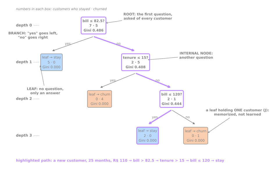
- A raiz é a primeira pergunta, feita a todo exemplo. Cada nó interno faz outra pergunta, só aos exemplos que chegaram até ele.
- Cada pergunta tem a forma atributo ≤ limiar. O ramo da esquerda é o "sim"; o da direita, o "não".
- Uma folha não pergunta nada: guarda uma resposta (a classe majoritária dos exemplos de treino que caíram nela) e as contagens que a justificam.
- A profundidade de um nó é o número de perguntas entre ele e a raiz; a profundidade da árvore é a do seu nó mais fundo.
- Prever é seguir um caminho: o cliente destacado tem conta de R$ 110 (não ≤ 82,5, vai à direita), 25 meses de casa (não ≤ 15, à direita) e conta ≤ 120 (à esquerda): "fica".
Repare na folha de baixo, à direita: ela guarda um único cliente. Guarde essa imagem; ela vai voltar na seção 4.
2. Impureza: quão misturado está um nó?
Um nó é um grupo de exemplos. Seja \(p_c\) a fração da classe \(c\) nele. Duas medidas clássicas de quão misturado ele está:
Impureza de Gini (o padrão do CART) — a probabilidade de que dois exemplos sorteados do nó, com reposição, sejam de classes diferentes:
Entropia (do ID3 e do C4.5 de Quinlan) — o número médio de bits necessários para codificar a classe de um exemplo sorteado do nó:
As duas valem 0 num nó puro (uma só classe) e são máximas numa mistura equilibrada: com duas classes, \(G = 0{,}5\) e \(H = 1\) em 50/50. Na raiz da nossa tabela, 7 ficaram e 5 cancelaram:
def gini(y):
    p = np.bincount(y, minlength=2) / len(y)
    return 1 - np.sum(p ** 2)

def entropy(y):
    p = np.bincount(y, minlength=2) / len(y)
    p = p[p > 0]
    return -np.sum(p * np.log2(p))

y_c = customers['churn'].to_numpy()
print(f"root: Gini {gini(y_c):.3f} · entropy {entropy(y_c):.3f}")
3. A melhor pergunta: todos os cortes, pontuados
Etapa 2. Uma pergunta atributo ≤ t divide um nó de \(n\) exemplos num filho esquerdo com \(n_L\) e num filho direito com \(n_R\). O corte é pontuado pela impureza ponderada dos filhos; seu ganho é o quanto ela fica abaixo da impureza do pai:
Com a entropia no papel de \(I\), \(\Delta\) se chama ganho de informação. Os pesos importam: um filho puro com um único exemplo não deve contar tanto quanto um filho puro com seis.
Quais limiares vale a pena testar? Entre dois valores distintos consecutivos do atributo, qualquer limiar produz o mesmo corte, então basta um por intervalo; o CART usa o ponto médio. As 12 contas têm 12 valores distintos, logo 11 candidatos:
def candidate_splits(feature):
    x = customers[feature].to_numpy()
    values = np.unique(x)                               # valores distintos, ordenados
    rows = []
    for t in (values[:-1] + values[1:]) / 2:            # pontos médios entre vizinhos
        left, right = y_c[x <= t], y_c[x > t]
        weighted = (len(left) * gini(left) + len(right) * gini(right)) / len(y_c)
        rows.append({'threshold': t,
                     'left (stay/churn)': f"{(left == 0).sum()}/{(left == 1).sum()}",
                     'right (stay/churn)': f"{(right == 0).sum()}/{(right == 1).sum()}",
                     'Gini left': gini(left), 'Gini right': gini(right),
                     'weighted Gini': weighted, 'decrease': gini(y_c) - weighted})
    return pd.DataFrame(rows)

table = candidate_splits('bill')
print(table.round(3).to_string(index=False))
best_tenure = candidate_splits('tenure').sort_values('weighted Gini').iloc[0]
print(f"best split on tenure: tenure <= {best_tenure['threshold']:g}, "
      f"weighted Gini {best_tenure['weighted Gini']:.3f}")
 threshold left (stay/churn) right (stay/churn)  Gini left  Gini right  weighted Gini  decrease
      50.0               1/0                6/5      0.000       0.496          0.455     0.032
      57.5               2/0                5/5      0.000       0.500          0.417     0.069
      62.5               3/0                4/5      0.000       0.494          0.370     0.116
      67.5               4/0                3/5      0.000       0.469          0.312     0.174
      82.5               5/0                2/5      0.000       0.408          0.238     0.248
      97.5               5/1                2/4      0.278       0.444          0.361     0.125
     105.0               6/1                1/4      0.245       0.320          0.276     0.210
     112.5               6/2                1/3      0.375       0.375          0.375     0.111
     117.5               7/2                0/3      0.346       0.000          0.259     0.227
     122.5               7/3                0/2      0.420       0.000          0.350     0.136
     127.5               7/4                0/1      0.463       0.000          0.424     0.062
best split on tenure: tenure <= 4, weighted Gini 0.350
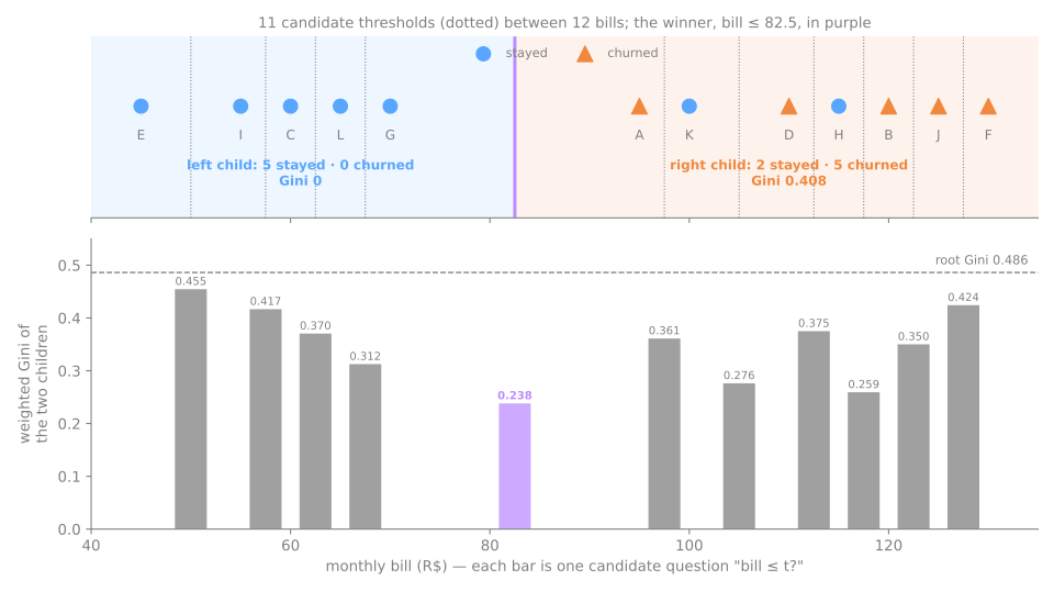
Confira a linha vencedora com uma calculadora. bill ≤ 82.5 (o ponto médio entre R$ 70 e R$ 95) manda para a esquerda os 5 clientes de conta mais baixa e todos eles ficaram: Gini 0. O filho direito tem 2 que ficaram e 5 que cancelaram:
Nenhum outro limiar em bill chega perto; a melhor pergunta sobre tenure (tenure ≤ 4, Gini ponderado 0,350) também é pior. Repare que a queda não é monótona ao longo da tabela: bill ≤ 97.5 (0,125) é bem pior que os vizinhos, porque leva um cliente que cancelou para o filho esquerdo e estraga a pureza dele. O único jeito de achar o melhor corte é pontuar todos.
A figura mostra a busca inteira de uma vez: os 12 clientes em ordem de conta, os 11 limiares candidatos entre eles e a nota de cada um (script da figura):
O scikit-learn concorda
Uma árvore limitada a um único corte se chama toco (stump). DecisionTreeClassifier(max_depth=1) precisa encontrar exatamente o corte acima:
from sklearn.tree import DecisionTreeClassifier, export_text

X_c = customers[['tenure', 'bill']]
stump = DecisionTreeClassifier(max_depth=1, random_state=0).fit(X_c, y_c)
t = stump.tree_
print("feature:", X_c.columns[t.feature[0]], "· threshold:", t.threshold[0])
print("node impurities (root, left, right):", t.impurity.round(3))
print(export_text(stump, feature_names=list(X_c.columns), show_weights=True))
stump_H = DecisionTreeClassifier(max_depth=1, criterion='entropy', random_state=0).fit(X_c, y_c)
print("with entropy:", X_c.columns[stump_H.tree_.feature[0]], "<=", stump_H.tree_.threshold[0],
      "· node entropies", stump_H.tree_.impurity.round(3))
feature: bill · threshold: 82.5
node impurities (root, left, right): [0.486 0.    0.408]
|--- bill <= 82.50
|   |--- weights: [5.00, 0.00] class: 0
|--- bill >  82.50
|   |--- weights: [2.00, 5.00] class: 1

with entropy: bill <= 82.5 · node entropies [0.98  0.    0.863]
Mesmo atributo, mesmo limiar, os mesmos três valores de Gini (0,486, 0, 0,408). A árvore ajustada mora em tree_: vetores paralelos indexados pelo número do nó, com feature, threshold, impurity, n_node_samples e value de cada nó. export_text a imprime como regras indentadas; show_weights=True acrescenta as contagens de classe em cada folha (ficou, cancelou). Com criterion='entropy' o toco escolhe o mesmo corte, com ganho de informação \(0{,}980 - \tfrac{7}{12}\cdot 0{,}863 = 0{,}476\). É o desfecho habitual: na prática, Gini e entropia discordam numa pequena fração dos cortes (Raileanu & Stoffel, 2004); o Gini é um pouco mais barato de calcular porque não precisa de logaritmo.
4. Crescendo a árvore
Guloso e recursivo
Etapa 3. O CART cresce a árvore inteira repetindo a busca do toco dentro de cada filho:
GROW(node):
    if a stopping rule holds (node is pure, max_depth reached, too few samples): make a leaf
    for each feature j, for each midpoint t between consecutive values of j:
        score the split x_j <= t by the impurity decrease Δ
    apply the best split; GROW(left child); GROW(right child)
Duas palavras o descrevem. Recursivo: cada filho é uma versão menor do mesmo problema. Guloso: cada corte é o melhor agora, sem olhar adiante; um corte que parece fraco sozinho, mas que abriria caminho para um corte excelente abaixo dele, nunca é escolhido. Encontrar a árvore globalmente ótima é NP-completo (Hyafil & Rivest, 1976), por isso todo algoritmo prático é guloso. Ele também é rápido: com os valores de cada atributo ordenados uma vez, pontuar todos os limiares de um nó custa uma passada pelas suas linhas; crescer uma árvore custa da ordem de \(O(p\, n \log n)\) para \(n\) linhas e \(p\) atributos.
Na tabela de churn, o filho esquerdo (bill ≤ 82.5) é puro e vira folha. O filho direito (2 ficaram, 5 cancelaram) é dividido de novo:
tree2 = DecisionTreeClassifier(max_depth=2, random_state=0).fit(X_c, y_c)
print(export_text(tree2, feature_names=list(X_c.columns), show_weights=True))

new = pd.DataFrame({'tenure': [6, 4, 25], 'bill': [70, 115, 110]}, index=['M', 'N', 'O'])
print(pd.DataFrame(tree2.predict_proba(new), index=new.index, columns=['P(stay)', 'P(churn)']).round(3)
      .assign(prediction=tree2.predict(new), leaf=tree2.apply(new)))
|--- bill <= 82.50
|   |--- weights: [5.00, 0.00] class: 0
|--- bill >  82.50
|   |--- tenure <= 15.00
|   |   |--- weights: [0.00, 4.00] class: 1
|   |--- tenure >  15.00
|   |   |--- weights: [2.00, 1.00] class: 0

   P(stay)  P(churn)  prediction  leaf
M    1.000     0.000           0     1
N    0.000     1.000           1     3
O    0.667     0.333           0     4
Dentro do grupo de conta alta, a melhor pergunta é tenure ≤ 15: os 4 clientes recentes com conta alta cancelaram todos. A árvore e a partição do plano que ela define (script da figura):
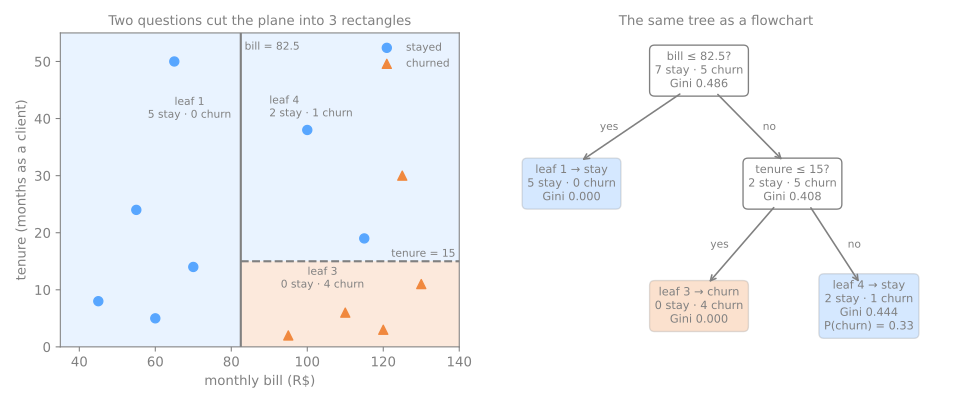
Todo corte é uma reta vertical ou horizontal que só corta a região do seu próprio nó: a reta tenure = 15 para em bill = 82.5. Assim, uma árvore sempre particiona o espaço de atributos em retângulos alinhados aos eixos (caixas, em mais dimensões), um por folha. O modelo também é uma afirmação sobre interações: o tempo de casa importa, mas só para clientes de conta alta. Um modelo linear precisaria de um atributo-produto explícito para dizer isso; a árvore o diz aninhando uma pergunta dentro da outra.
Folhas guardam proporções
Olhe os três clientes novos. M (conta 70) cai na folha 1, onde os 5 clientes de treino ficaram: P(churn) = 0. N (4 meses, R$ 115) cai na folha 3, onde os 4 cancelaram. O (25 meses, R$ 110) cai na folha 4, que guarda 2 que ficaram e 1 que cancelou: predict_proba devolve as proporções de classe dos exemplos de treino daquela folha, \((2/3, 1/3)\); predict devolve a maioria, "fica". apply informa o número da folha (os números de nó usados na figura acima). Todo exemplo de uma folha recebe a mesma probabilidade, então uma árvore com 3 folhas só consegue produzir 3 probabilidades distintas; a curva ROC de um modelo assim (aula de ROC e dados desbalanceados) tem poucos cantos.
Crescida até a pureza
A folha 4 ainda está misturada. Sem regra de parada, o CART continua dividindo até toda folha ficar pura:
full = DecisionTreeClassifier(random_state=0).fit(X_c, y_c)
print(export_text(full, feature_names=list(X_c.columns), show_weights=True))
print(f"leaves: {full.get_n_leaves()} · depth: {full.get_depth()} · training accuracy: {full.score(X_c, y_c):.3f}")
|--- bill <= 82.50
|   |--- weights: [5.00, 0.00] class: 0
|--- bill >  82.50
|   |--- tenure <= 15.00
|   |   |--- weights: [0.00, 4.00] class: 1
|   |--- tenure >  15.00
|   |   |--- bill <= 120.00
|   |   |   |--- weights: [2.00, 0.00] class: 0
|   |   |--- bill >  120.00
|   |   |   |--- weights: [0.00, 1.00] class: 1

leaves: 4 · depth: 3 · training accuracy: 1.000
A terceira pergunta, bill ≤ 120, existe para isolar um único cliente: J, com 30 meses de casa, que cancelou pagando R$ 125. "Clientes antigos acima de R$ 120 cancelam" é um padrão ou um acidente de uma linha? Com um só exemplo não há como saber; a árvore nem se pergunta e chega a 100% de acurácia de treino porque tem permissão para isso. Guarde esta imagem: ela é toda a história do sobreajuste desta aula, em miniatura.
A figura junta os quatro estágios, do nó único à árvore pura, com o número de folhas e a acurácia de treino de cada um (script da figura):
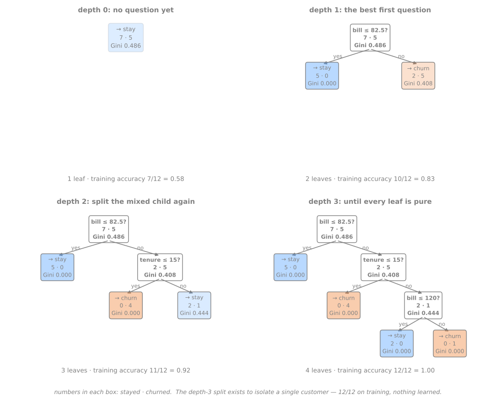
A acurácia de treino sobe a cada nível: 0,58, 0,83, 0,92 e, por fim, 1,00. Os dois primeiros cortes separam grupos de 5 e de 4 clientes; o terceiro existe por causa de um cliente. Uma acurácia de treino perfeita, numa árvore sem limite, não é uma conquista: é o que o algoritmo sempre faz.
O simulador cresce uma árvore um nível por vez em 120 pontos. Aumente a profundidade e veja as regiões se estilhaçarem em caixinhas em volta de pontos isolados, enquanto a impureza de treino continua caindo:
5. Sobreajuste e pré-poda
Uma árvore crescida até o fim memoriza
Etapa 4. A tabela de 12 clientes sugeriu; um conjunto real mede. O Spambase (Hopkins et al., 1999) tem 4.601 e-mails descritos por 57 números: frequências de palavras (word_freq_free, word_freq_hp), de caracteres (char_freq_$, char_freq_!) e sequências de letras maiúsculas. A tarefa é sinalizar spam. A divisão desenvolvimento/teste e o objeto cv abaixo são reutilizados no resto da aula:
from sklearn.datasets import fetch_openml
from sklearn.model_selection import StratifiedKFold, cross_validate, train_test_split
from urllib.parse import unquote

spam = fetch_openml(data_id=44, as_frame=True)          # Spambase: 4.601 e-mails, 57 atributos
X, y = spam.data, spam.target.astype(int)               # 1 = spam
X.columns = [unquote(c) for c in X.columns]             # 'char_freq_%24' -> 'char_freq_$'
repeated = X.duplicated()
print(f"{repeated.sum()} rows repeat an earlier row exactly: dropped")
X, y = X[~repeated], y[~repeated]
X_dev, X_test, y_dev, y_test = train_test_split(X, y, test_size=0.25, stratify=y, random_state=0)
print(X_dev.shape, X_test.shape, f"spam share {y_dev.mean():.3f}")

cv = StratifiedKFold(n_splits=5, shuffle=True, random_state=0)
res = cross_validate(DecisionTreeClassifier(random_state=0), X_dev, y_dev, cv=cv,
                     return_train_score=True, return_estimator=True)
print(f"training folds {res['train_score'].mean():.3f} · validation folds "
      f"{res['test_score'].mean():.3f} ± {res['test_score'].std():.3f}")
print("leaves per fold:", [int(m.get_n_leaves()) for m in res['estimator']],
      "· depth per fold:", [int(m.get_depth()) for m in res['estimator']])
394 rows repeat an earlier row exactly: dropped
(3155, 57) (1052, 57) spam share 0.399
training folds 1.000 · validation folds 0.906 ± 0.008
leaves per fold: [171, 187, 181, 188, 179] · depth per fold: [32, 28, 31, 30, 27]
Primeiro, 394 e-mails aparecem duas vezes com atributos idênticos. Se ficassem, uma cópia num fold de validação seria "prevista" pela sua gêmea nos folds de treino — o vazamento por linhas duplicadas da aula de validação. Um modelo que memoriza, como uma árvore crescida até o fim, seria o que mais lucraria com isso. Por isso, nós as descartamos.
Depois, a medida: a árvore crescida até o fim tem 1,000 nos folds de treino e 0,906 nos de validação. Para chegar lá ela precisa de cerca de 180 folhas e profundidade perto de 30 para uns 2.500 e-mails: muitas folhas guardam um ou dois e-mails de treino, exatamente como a folha que isolava o cliente J acima. Árvores são modelos de baixo viés e alta variância: nada no algoritmo interrompe a recursão antes de toda folha ficar pura — e uma folha pura é um exemplo memorizado. Existem duas famílias de remédios.
Pré-poda: parar cedo
Regras de parada encerram a recursão antes de as folhas ficarem puras. Os principais botões do DecisionTreeClassifier:
max_depth— o caminho mais longo da raiz até uma folha;min_samples_leaf— toda folha precisa manter pelo menos este número de exemplos de treino (um corte que criaria um filho menor não é permitido);max_leaf_nodes— cresce pelo melhor corte primeiro e para neste número de folhas;min_samples_split,min_impurity_decrease— não divide nós pequenos nem cortes que ganham pouco demais.
settings = [{}, {'max_depth': 3}, {'max_depth': 10},
            {'min_samples_leaf': 5}, {'min_samples_leaf': 50},
            {'max_leaf_nodes': 8}, {'max_leaf_nodes': 40}]
rows = []
for s in settings:
    r = cross_validate(DecisionTreeClassifier(random_state=0, **s), X_dev, y_dev, cv=cv,
                       return_train_score=True, return_estimator=True)
    rows.append({'setting': str(s) if s else 'none (fully grown)',
                 'train': r['train_score'].mean(), 'validation': r['test_score'].mean(),
                 'std': r['test_score'].std(),
                 'leaves': np.mean([m.get_n_leaves() for m in r['estimator']])})
print(pd.DataFrame(rows).round(3).to_string(index=False))
                 setting  train  validation   std  leaves
      none (fully grown)  1.000       0.906 0.008   181.2
        {'max_depth': 3}  0.890       0.880 0.012     8.0
       {'max_depth': 10}  0.967       0.915 0.009    86.4
 {'min_samples_leaf': 5}  0.957       0.900 0.006   111.8
{'min_samples_leaf': 50}  0.902       0.892 0.012    30.4
   {'max_leaf_nodes': 8}  0.899       0.891 0.007     8.0
  {'max_leaf_nodes': 40}  0.950       0.906 0.004    40.0
Todo botão move a árvore ao longo do mesmo eixo de viés–variância. Apertado demais (max_depth=3, 8 folhas) e as acurácias de treino e de validação são ambas baixas, 0,890 e 0,880: subajuste, visível porque os dois números andam juntos. Frouxo demais (sem limite) e a acurácia de treino chega a 1,000 enquanto a de validação fica em 0,906. No meio, max_depth=10 chega a 0,915 com 86 folhas. A linha mais marcante é max_leaf_nodes=40: a mesma acurácia de validação da árvore crescida até o fim (0,906) com 40 folhas em vez de 181. As outras 140 folhas foram gastas memorizando.
6. Lendo uma árvore: um caminho é uma regra
Etapa 5. A principal razão para usar uma árvore sozinha em vez de um ensemble é que uma pessoa consegue lê-la. Uma árvore de profundidade 2 no Spambase:
small = DecisionTreeClassifier(max_depth=2, random_state=0).fit(X_dev, y_dev)
print(export_text(small, feature_names=list(X.columns), show_weights=True))
print(f"test accuracy of this 4-leaf tree: {small.score(X_test, y_test):.3f}")
|--- char_freq_$ <= 0.05
|   |--- word_freq_remove <= 0.06
|   |   |--- weights: [1770.00, 356.00] class: 0
|   |--- word_freq_remove >  0.06
|   |   |--- weights: [19.00, 211.00] class: 1
|--- char_freq_$ >  0.05
|   |--- word_freq_hp <= 0.38
|   |   |--- weights: [50.00, 687.00] class: 1
|   |--- word_freq_hp >  0.38
|   |   |--- weights: [57.00, 5.00] class: 0

test accuracy of this 4-leaf tree: 0.863
Cada caminho da raiz até uma folha é uma regra se–então; os pesos dizem quantos dados de treino a sustentam (não spam, spam):
- se
$é raro (≤ 0,05% dos caracteres) eremoveé raro: não é spam — 1.770 e-mails legítimos contra 356 spams; - se
$é raro masremoveaparece (como em "clique aqui para ser removido da lista"): spam, 211 contra 19; - se
$é frequente ehpé raro: spam, 687 contra 50; - se
$é frequente mashpaparece: não é spam, 57 contra 5. Os dados foram coletados na Hewlett-Packard; uma mensagem que mencionahpera, muito provavelmente, correio interno.
Quatro regras, 0,863 no teste: 6 pontos abaixo da árvore crescida até o fim (0,923 no teste, como a seção 12 vai medir), com 4 folhas em vez de 221 e um modelo que qualquer um pode conferir. A última regra também mostra por que ler importa: ela é verdadeira neste conjunto de dados e inútil em qualquer outro lugar — e só olhando você descobre isso. plot_tree desenha a mesma árvore como diagrama (você vai usá-lo no lab).
7. Resumo: uma árvore em cinco linhas
- Uma árvore faz perguntas atributo ≤ limiar, uma de cada vez, da raiz até uma folha; prever é seguir um caminho.
- Uma boa pergunta deixa os filhos mais puros. A impureza (Gini ou entropia) mede a mistura; um corte é pontuado pela impureza ponderada dos filhos.
- O melhor corte é achado por força bruta: todos os atributos, todos os pontos médios entre valores vizinhos.
- O crescimento é guloso e recursivo: o melhor corte agora, repetido dentro de cada filho, até uma regra de parada.
- Sem regra de parada, a árvore decora: folhas puras, treino perfeito.
max_depth,min_samples_leafemax_leaf_nodesa seguram; a validação cruzada escolhe quanto.
| sintoma | o que está acontecendo | o que fazer |
|---|---|---|
| acurácia de treino 1,000, validação bem abaixo | a árvore decorou o treino | limitar profundidade ou tamanho de folha |
| treino e validação baixos e parecidos | a árvore é rasa demais | deixar crescer mais um nível |
| centenas de folhas para alguns milhares de linhas | folhas com um ou dois exemplos | min_samples_leaf ou max_leaf_nodes |
| uma árvore pequena acerta quase tanto quanto a grande | as folhas extras só memorizavam | ficar com a pequena: ela se lê |
Lab fundamental — uma chave para pinguins
O problema. Guias de campo identificam espécies com uma chave dicotômica: uma lista de perguntas de sim ou não ("bico com mais de 43 mm? vá para 5; senão, vá para 7") que termina no nome de uma espécie. Uma chave dicotômica é uma árvore de decisão escrita à mão. O conjunto Palmer penguins (Gorman et al., 2014) tem 344 pinguins de três espécies, Adelie, Chinstrap e Gentoo, medidos em três ilhas do Arquipélago Palmer, na Antártida: comprimento e profundidade do bico (culmen), comprimento da nadadeira, massa corporal, sexo e ilha. A equipe de campo quer uma chave pequena o bastante para caber num cartão e quer saber quanto essa legibilidade custa em acurácia, comparada a modelos que ninguém consegue ler.
O fluxo é o da aula de validação: trancar um conjunto de teste, usar um único objeto cv para tudo e tocar o teste uma única vez, no passo 8. Esta parte prepara os dados, constrói e lê uma chave de profundidade 2 e deixa a árvore crescer até o fim; o ajuste, a comparação com outros modelos e o teste ficam para o lab avançado.
Como fazer este lab em aula (cerca de 30 min, em duplas)
- Abra o notebook do lab no Colab. Não é preciso baixar nem instalar nada: o Colab roda no navegador. Para guardar as suas respostas, salve uma cópia no seu Drive (Arquivo → Salvar uma cópia no Drive) antes de editar. Rode as células em ordem, numa mesma sessão.
- Este lab corresponde aos passos 1 a 5 do notebook. O lab avançado continua no mesmo notebook, a partir do passo 6.
- Cada passo começa com um Preveja: responda com a dupla antes de rodar a célula. Errar a previsão é o que torna o resultado memorável.
- Depois de rodar, compare com a saída e a leitura desta página. Toda saída aqui é exatamente o que o código imprime.
- As Simulações pedem que vocês escrevam um pequeno experimento em Python: mudar uma entrada e observar o que acontece com a saída. Nada de conta à mão. A solução fica recolhida logo abaixo: tente antes de abrir.
- Ritmo sugerido: passos 1 a 3 em 8 min; passo 4 e a primeira simulação em 12 min; passo 5 e a segunda simulação em 10 min.
Passo 1 — carregar e olhar
Preveja. São três espécies de pinguins. Você espera que elas apareçam em proporções parecidas? Que acurácia teria um modelo que sempre responde a espécie mais comum?
import numpy as np
import pandas as pd
from sklearn.datasets import fetch_openml

peng = fetch_openml(data_id=42585, as_frame=True).frame      # Palmer penguins
print(peng.shape)
print(peng['species'].value_counts().to_dict())
print(peng.isna().sum().to_dict())
print(peng['sex'].value_counts(dropna=False).to_dict())
(344, 7)
{'Adelie': 152, 'Gentoo': 124, 'Chinstrap': 68}
{'species': 0, 'island': 0, 'culmen_length_mm': 2, 'culmen_depth_mm': 2, 'flipper_length_mm': 2, 'body_mass_g': 2, 'sex': 10}
{'MALE': 168, 'FEMALE': 165, nan: 10, '_': 1}
344 pinguins: 152 Adelie, 124 Gentoo e só 68 Chinstrap, então a acurácia precisa ser lida contra um baseline majoritário de 44%. Duas aves não têm medida nenhuma. A coluna sex tem 10 valores faltantes e uma entrada, '_', que não é nenhum dos sexos: um erro de digitação, a ser tratado como faltante.
Passo 2 — limpar e codificar
Preveja. A árvore aceita NaN e não precisa de escalonamento. Das três limpezas de costume — imputar, escalonar, codificar categorias —, qual ainda é necessária aqui?
num = ['culmen_length_mm', 'culmen_depth_mm', 'flipper_length_mm', 'body_mass_g']
peng = peng.dropna(subset=num)                    # as 2 aves sem medida nenhuma
X = peng[num].copy()
X['is_male'] = peng['sex'].astype(object).map({'MALE': 1.0, 'FEMALE': 0.0})   # '_' e desconhecido -> NaN
X = X.join(pd.get_dummies(peng['island'], prefix='island', dtype=float))      # one-hot
y = peng['species'].astype(str)
print(X.shape)
print("missing:", X.isna().sum()[X.isna().sum() > 0].to_dict())
print(X.head(3).to_string())
(342, 8)
missing: {'is_male': 9}
   culmen_length_mm  culmen_depth_mm  flipper_length_mm  body_mass_g  is_male  island_Biscoe  island_Dream  island_Torgersen
0              39.1             18.7              181.0       3750.0      1.0            0.0           0.0               1.0
1              39.5             17.4              186.0       3800.0      0.0            0.0           0.0               1.0
2              40.3             18.0              195.0       3250.0      0.0            0.0           0.0               1.0
342 pinguins e 8 colunas numéricas. island é categórica, então vira três colunas 0/1 (one-hot). sex vira is_male, com NaN para os 9 pinguins restantes de sexo desconhecido. Mantemos esses NaN: a árvore os aceita como estão; os rivais do passo 7 vão ganhar um imputador dentro dos seus pipelines. Nada é escalonado; a árvore não precisa.
Passo 3 — trancar o conjunto de teste e um baseline
Preveja. Com 86 pinguins no teste, quanto vale um único erro em pontos de acurácia? Isso muda o quanto você deve confiar na terceira casa decimal?
from sklearn.dummy import DummyClassifier
from sklearn.model_selection import StratifiedKFold, cross_validate, train_test_split

X_train, X_test, y_train, y_test = train_test_split(X, y, test_size=0.25, stratify=y, random_state=42)
print(X_train.shape, X_test.shape)

cv = StratifiedKFold(n_splits=5, shuffle=True, random_state=42)


def cv_report(model):
    r = cross_validate(model, X_train, y_train, cv=cv, return_train_score=True)
    return (f"train {r['train_score'].mean():.3f} · validation "
            f"{r['test_score'].mean():.3f} ± {r['test_score'].std():.3f}")


print("dummy:", cv_report(DummyClassifier(strategy='most_frequent')))
256 pinguins para desenvolvimento e 86 trancados até o passo 8, com as proporções de espécies preservadas por stratify=y. Com 86 aves de teste, um erro custa 1,2 ponto de acurácia. Responder sempre "Adelie" dá 0,441. cv_report imprime a acurácia média de treino e de validação nos mesmos cinco folds, que todos os passos seguintes reutilizam.
Passo 4 — uma árvore de profundidade 2, lida como regras
Preveja. Uma única pergunta (profundidade 1) consegue separar três espécies? E, com duas perguntas em sequência, que medida você acha que a raiz vai usar?
import matplotlib.pyplot as plt
from sklearn.tree import DecisionTreeClassifier, export_text, plot_tree

print("depth 1:", cv_report(DecisionTreeClassifier(max_depth=1, random_state=0)))
print("depth 2:", cv_report(DecisionTreeClassifier(max_depth=2, random_state=0)))

tree2 = DecisionTreeClassifier(max_depth=2, random_state=0).fit(X_train, y_train)
print(tree2.classes_)
print(export_text(tree2, feature_names=list(X.columns), show_weights=True))

plot_tree(tree2, feature_names=list(X.columns), class_names=list(tree2.classes_),
          filled=True, rounded=True, fontsize=8)
plt.show()
depth 1: train 0.785 · validation 0.770 ± 0.034
depth 2: train 0.960 · validation 0.938 ± 0.040
['Adelie' 'Chinstrap' 'Gentoo']
|--- flipper_length_mm <= 206.50
|   |--- culmen_length_mm <= 43.35
|   |   |--- weights: [107.00, 4.00, 0.00] class: Adelie
|   |--- culmen_length_mm >  43.35
|   |   |--- weights: [4.00, 42.00, 1.00] class: Chinstrap
|--- flipper_length_mm >  206.50
|   |--- culmen_depth_mm <= 17.55
|   |   |--- weights: [0.00, 0.00, 91.00] class: Gentoo
|   |--- culmen_depth_mm >  17.55
|   |   |--- weights: [2.00, 5.00, 0.00] class: Chinstrap
Como ler:
- Uma pergunta não basta. Um toco só pode ter duas folhas, então só consegue nomear duas das três espécies: 0,770.
- Dois níveis já fazem uma chave utilizável, 0,938 ± 0,040, com quatro regras. Os pesos são as contagens de (Adelie, Chinstrap, Gentoo) em cada folha. Nadadeira longa (> 206,5 mm) e bico raso (≤ 17,55 mm) é Gentoo: 91 de 91. Nadadeira curta e bico curto (≤ 43,35 mm) é Adelie: 107 de 111. Nadadeira curta e bico longo é Chinstrap: 42 de 47.
- Os erros ficam onde as espécies se sobrepõem. Adelie e Chinstrap têm nadadeiras parecidas e diferem principalmente no comprimento do bico: 8 das 9 aves mal classificadas nas duas folhas da esquerda são Adelies e Chinstraps do lado errado do limiar de 43,35 mm. A quarta folha (nadadeira longa, bico fundo) guarda só 7 aves, uma mistura de Adelie e Chinstrap.
plot_tree desenha a mesma árvore; cada caixa mostra a pergunta, o Gini do nó, o número de amostras, as contagens de classe (value) e a classe majoritária, colorida pela classe e pela pureza.
Simulação: a raiz, escolhida por você. A seção 3 pontuou à mão todos os cortes de uma tabela de 12 clientes. Faça o mesmo com os pinguins: para cada uma das quatro medidas, teste todos os pontos médios entre valores vizinhos em X_train, pontue cada corte pelo Gini ponderado (agora com três classes) e guarde o melhor. A pergunta vencedora é a raiz que a árvore do passo 4 escolheu? Por quanto ela vence?
Solução
def gini_counts(labels):
    p = labels.value_counts(normalize=True).to_numpy()     # frações das espécies no nó
    return 1 - np.sum(p ** 2)

print(f"root Gini: {gini_counts(y_train):.3f}")
for col in ['culmen_length_mm', 'culmen_depth_mm', 'flipper_length_mm', 'body_mass_g']:
    x = X_train[col].to_numpy()
    values = np.unique(x)
    best = (np.inf, None)
    for t in (values[:-1] + values[1:]) / 2:               # pontos médios entre vizinhos
        left, right = y_train[x <= t], y_train[x > t]
        w = (len(left) * gini_counts(left) + len(right) * gini_counts(right)) / len(y_train)
        best = min(best, (w, t))
    print(f"{col:18s} {len(values) - 1:3d} thresholds · best <= {best[1]:7.2f} · weighted Gini {best[0]:.3f}")
root Gini: 0.636
culmen_length_mm   144 thresholds · best <=   42.30 · weighted Gini 0.324
culmen_depth_mm     75 thresholds · best <=   16.40 · weighted Gini 0.331
flipper_length_mm   51 thresholds · best <=  206.50 · weighted Gini 0.312
body_mass_g         89 thresholds · best <= 4525.00 · weighted Gini 0.400
Foram 359 perguntas candidatas (144 + 75 + 51 + 89) e a vencedora é exatamente a raiz do passo 4, flipper_length_mm <= 206.50, com Gini ponderado 0,312. Mas a vitória é apertada: o melhor corte no comprimento do bico fica em 0,324 e o melhor na profundidade, em 0,331. Três perguntas quase igualmente boas disputam a raiz, então uma pequena mudança nos dados pode trocar a vencedora — guarde isso para o passo 10. A massa corporal (0,400) separa bem pior: pesar a ave não basta. E, com três classes, o Gini da raiz é 0,636, acima do máximo de 0,5 que ele atinge com duas: com \(K\) classes equilibradas, o máximo é \(1 - 1/K\).
Passo 5 — crescer até o fim
Preveja. Sem limite nenhum, a árvore chega a 100% de acurácia no treino? E na validação: ela vai piorar em relação à de profundidade 2, como no Spambase, ou melhorar?
full = DecisionTreeClassifier(random_state=0)
print("fully grown:", cv_report(full))
full.fit(X_train, y_train)
print(f"depth {full.get_depth()} · {full.get_n_leaves()} leaves for {len(X_train)} penguins")
A árvore crescida até o fim ajusta perfeitamente os folds de treino (1,000) e marca 0,969 ± 0,016 na validação, melhor que a de profundidade 2. Ao contrário do Spambase, os pinguins são fáceis e limpos: a árvore completa precisa de só 13 folhas, então há pouco para memorizar. Mas 13 folhas não cabem num cartão.
Simulação: uma árvore decora até rótulos aleatórios. Embaralhe as espécies de y_train — cada pinguim fica com a espécie de outro, sorteado — e repita a validação cruzada da árvore crescida até o fim. O que acontece com a acurácia de treino? E com a de validação? Compare também o número de folhas com o da árvore com os rótulos verdadeiros.
Solução
shuffled = y_train.sample(frac=1, random_state=0).to_numpy()      # as espécies, embaralhadas
r = cross_validate(DecisionTreeClassifier(random_state=0), X_train, shuffled, cv=cv,
                   return_train_score=True, return_estimator=True)
print(f"random labels: train {r['train_score'].mean():.3f} · validation {r['test_score'].mean():.3f}"
      f" · {np.mean([m.get_n_leaves() for m in r['estimator']]):.0f} leaves for ~205 penguins")
print(f"real labels:   {cv_report(full)}")
random labels: train 1.000 · validation 0.355 · 84 leaves for ~205 penguins
real labels:   train 1.000 · validation 0.969 ± 0.016
Com rótulos aleatórios não há nada para aprender e, mesmo assim, a árvore chega a 1,000 nos folds de treino: ela cresce até cada folha ficar pura, custe o que custar — 84 folhas para uns 205 pinguins por fold, contra 13 da árvore do passo 5 com todos os 256. A validação desaba para 0,355, abaixo até do baseline de 0,441: as regras decoradas não valem nada em pinguins novos. A lição: a acurácia de treino de uma árvore crescida até o fim não diz nada, porque ela é 1,000 com sinal ou sem sinal. Só a validação separa os dois casos; o número de folhas é um bom alarme.
Para fechar a parte fundamental. Em uma frase cada: (1) o que faz uma pergunta ser melhor que outra? (2) Por que uma árvore crescida até o fim chega a 100% de acurácia de treino, mesmo com rótulos aleatórios? (3) Como você leria em voz alta um caminho da raiz até uma folha da chave do passo 4?
Sua vez (fundamental)
Para casa:
- Entropia. Refaça o passo 4 com
criterion='entropy'. A árvore de profundidade 2 escolhe as mesmas perguntas? E os mesmos limiares? - O ganho de informação à mão. Na tabela dos 12 clientes, calcule à mão a entropia dos dois filhos de
bill ≤ 82.5e o ganho de informação do corte. Confira com o 0,476 da seção 3. - Folhas mínimas em vez de profundidade. Refaça o passo 5 com
min_samples_leaf=5e commin_samples_leaf=10. Quantas folhas a árvore tem e o que acontece com a acurácia de treino e com a de validação?
Abordagem avançada
A parte fundamental cresceu uma árvore e a impediu de decorar. Esta parte mostra onde as árvores brilham e onde falham: por que o critério de corte não pode ser a taxa de erro, como uma árvore faz regressão (e por que não extrapola), como podar depois de crescer, por que uma árvore muda tanto com os dados e o que ela dispensa — e não dispensa — em relação a outros modelos. Os blocos de código continuam os das seções 1 a 6.
Esta parte segue um caminho em quatro etapas, desenhado abaixo: 1. medir o corte; 2. podar depois de crescer; 3. encarar a instabilidade; 4. forças e limites. Cada etapa leva à sua seção e, nos slides, uma faixa embaixo mostra em que etapa você está.
- Medir o corteimpureza, não erros; variância na regressão
- Podar depois de crescerpoda por custo-complexidade e a escolha de α
- Encarar a instabilidadeuma pequena mudança nos dados, outra árvore
- Forças e limitesescala, escadas,
NaN, importância
Slides da abordagem avançada
Clique nos slides e use as setas ← → para navegar; F abre em tela cheia e Esc mostra todos os slides. Abrir os slides numa aba nova
8. Por que não simplesmente contar erros?
Etapa 1. A medida mais óbvia de quão misturado está um nó seria sua taxa de erro de classificação: a fração de exemplos que não são da classe majoritária, \(1 - \max_c p_c\). É o que no fim nos interessa, então por que não cortar com base nela? A figura mostra as três medidas lado a lado e um corte que expõe o problema (script da figura):
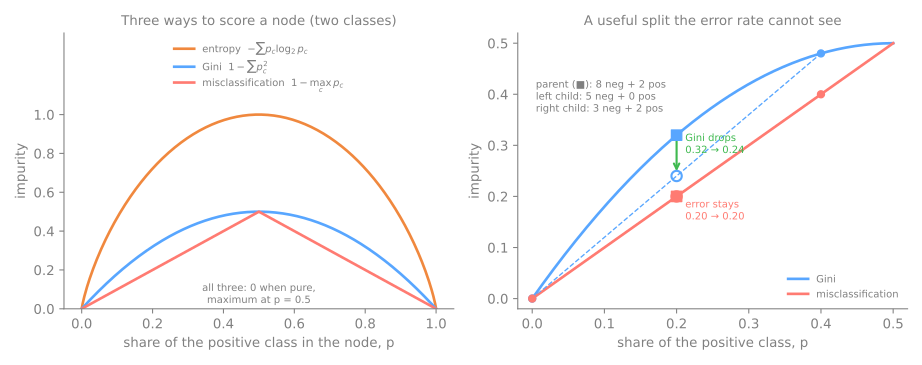
O pai tem 8 negativos e 2 positivos, então prevê "negativo" e erra 2 em 10. O corte manda 5 negativos para um filho esquerdo puro e deixa 3 negativos e 2 positivos à direita. Os dois filhos continuam prevendo "negativo" e o direito continua cometendo exatamente os mesmos 2 erros: a taxa de erro fica em \(0{,}20\) e o corte parece inútil. No entanto, é um bom primeiro passo: um filho está puro e resolvido; os positivos agora estão concentrados num nó de 5, onde a próxima pergunta pode isolá-los. O Gini enxerga esse progresso, caindo de \(0{,}32\) para \(\tfrac{5}{10}\cdot 0 + \tfrac{5}{10}\cdot 0{,}48 = 0{,}24\).
O painel da direita mostra o porquê geometricamente. A impureza ponderada dos filhos é um ponto sobre a corda que liga os pontos dos dois filhos, tomado no \(p\) do pai. A taxa de erro é uma reta entre 0 e 0,5, então a corda fica sobre a curva e a queda é zero. Gini e entropia são estritamente côncavas, então a corda fica abaixo da curva e todo corte que muda as proporções das classes mostra uma queda positiva. Crescer uma árvore é uma sequência de passos cujo valor muitas vezes só aparece um nível abaixo; um critério que recompensa o progresso (e não só as decisões acabadas) é o que faz a busca gulosa funcionar.
9. Árvores de regressão
Redução de variância, à mão
Para um alvo numérico, o mesmo algoritmo funciona com outra impureza. Uma folha prevê a média dos alvos de treino, então uma impureza natural é o erro quadrático médio em torno dessa média, que é a variância do alvo no nó:
O corte é pontuado exatamente como antes, pela impureza ponderada dos filhos. Oito apartamentos, área em m² e aluguel mensal em milhares de R$:
from sklearn.tree import DecisionTreeRegressor

flats = pd.DataFrame({'area': [30, 38, 45, 52, 60, 75, 90, 110],             # m²
                      'rent': [1.3, 1.5, 1.6, 2.0, 2.2, 3.1, 3.4, 3.8]})      # milhares de R$ / mês
area, rent = flats['area'].to_numpy(), flats['rent'].to_numpy()
mse = lambda v: np.mean((v - v.mean()) ** 2)                # impureza de um nó de regressão
print(f"root: mean {rent.mean():.3f} · MSE {mse(rent):.4f}")

rows = []
for t in (area[:-1] + area[1:]) / 2:
    left, right = rent[area <= t], rent[area > t]
    weighted = (len(left) * mse(left) + len(right) * mse(right)) / len(rent)
    rows.append({'threshold': t, 'mean left': left.mean(), 'mean right': right.mean(),
                 'weighted MSE': weighted, 'decrease': mse(rent) - weighted})
print(pd.DataFrame(rows).round(4).to_string(index=False))

reg = DecisionTreeRegressor(max_depth=1).fit(flats[['area']], rent)
print(export_text(reg, feature_names=['area'], decimals=3))
root: mean 2.362 · MSE 0.7873
 threshold  mean left  mean right  weighted MSE  decrease
      34.0     1.3000      2.5143        0.6261    0.1613
      41.5     1.4000      2.6833        0.4785    0.3088
      48.5     1.4667      2.9000        0.3058    0.4815
      56.0     1.6000      3.1250        0.2059    0.5814
      67.5     1.7200      3.4333        0.0993    0.6880
      82.5     1.9500      3.6000        0.2769    0.5105
     100.0     2.1571      3.8000        0.4921    0.2952
|--- area <= 67.500
|   |--- value: [1.720]
|--- area >  67.500
|   |--- value: [3.433]
Antes de qualquer corte, a melhor previsão constante é a média, R$ 2,362 mil, com MSE 0,7873. O corte area ≤ 67.5, que prevê R$ 1,720 mil para os cinco apartamentos pequenos e R$ 3,433 mil para os três grandes, derruba o MSE ponderado para 0,0993: uma única pergunta remove \(0{,}688 / 0{,}787 = 87\%\) da variância. O DecisionTreeRegressor encontra o mesmo limiar e os mesmos dois valores de folha.
Uma função em escada que não extrapola
Uma árvore de regressão com \(L\) folhas prevê no máximo \(L\) valores diferentes, então sua curva de previsão é uma função em escada. A figura ajusta árvores de profundidade 1 e 3 e uma regressão linear a 60 apartamentos entre 30 e 120 m² (a relação verdadeira é uma reta mais ruído) e as avalia em apartamentos novos dentro e fora dessa faixa (script da figura):
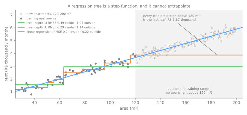
Dentro da faixa de treino, a escada de profundidade 3 acompanha a reta razoavelmente (RMSE 0,29 contra 0,24 do modelo linear, que tem a forma certa por construção). Fora dela, todo apartamento maior que 120 m² cai na última folha e recebe a mesma previsão, R$ 3,87 mil, por maior que seja: RMSE 1,14, cinco vezes o 0,22 do modelo linear. Uma árvore não extrapola: ela só consegue devolver médias de alvos que já viu. Isso pesa para vendas que crescem com o tempo, preços sob inflação ou qualquer alvo que precise ir além da faixa de treino. A limitação vale também para as florestas e os ensembles de boosting construídos com árvores.
10. Pós-poda: crescer, depois cortar
Etapa 2. As regras de parada têm uma fraqueza que vem da estratégia gulosa: um corte que ganha pouco pode abrir caminho para um grande ganho abaixo dele, algo que uma parada precoce nunca descobre. A resposta do CART (Breiman et al., 1984) é o procedimento inverso: crescer a árvore inteira e depois podá-la. A poda usa o critério de custo-complexidade, que cobra um preço \(\alpha\) por folha:
em que \(R(T)\) é a impureza total das folhas da árvore \(T\) (a impureza de cada folha ponderada pela sua fração das linhas de treino) e \(|T|\) é o número de folhas. É a versão para árvores da regularização: \(\alpha = 0\) mantém a árvore inteira; \(\alpha\) maior encarece as folhas. Para cada nó interno \(t\), colapsar sua subárvore \(T_t\) numa única folha economiza \(|T_t| - 1\) folhas e custa \(R(t) - R(T_t)\) de impureza, então compensa a partir de
A poda do elo mais fraco colapsa o nó de menor \(\alpha_{\text{ef}}\), recalcula e repete, produzindo uma sequência encaixada de subárvores até sobrar só a raiz. Na árvore completa de churn (4 folhas, todas puras, logo \(R(T) = 0\)), à mão:
- nó
bill ≤ 120(3 clientes: 2 ficaram, 1 cancelou; Gini 0,444): \(R(t) = \tfrac{3}{12}\cdot 0{,}444 = 0{,}111\), sua subárvore tem 2 folhas, então \(\alpha_{\text{ef}} = 0{,}111 / 1 = 0{,}111\); - nó
tenure ≤ 15(7 clientes, Gini 0,408): \(R(t) = \tfrac{7}{12}\cdot 0{,}408 = 0{,}238\), 3 folhas: \(0{,}238 / 2 = 0{,}119\); - a raiz: \(0{,}486 / 3 = 0{,}162\).
O elo mais fraco é bill ≤ 120, podado em \(\alpha = 0{,}111\), o que remove exatamente o corte que isolava o cliente J. Recalculando na árvore de 3 folhas, tenure ≤ 15 agora economiza uma folha por \(0{,}238 - 0{,}111 = 0{,}127\); a raiz sai por último, em \(0{,}486 - 0{,}238 = 0{,}248\). O scikit-learn calcula a mesma sequência:
path_c = DecisionTreeClassifier(random_state=0).cost_complexity_pruning_path(X_c, y_c)
for a, imp in zip(path_c.ccp_alphas, path_c.impurities):
    leaves = DecisionTreeClassifier(random_state=0, ccp_alpha=a).fit(X_c, y_c).get_n_leaves()
    print(f"ccp_alpha {a:.3f} -> {leaves} leaves, total leaf impurity {imp:.3f}")
ccp_alpha 0.000 -> 4 leaves, total leaf impurity 0.000
ccp_alpha 0.111 -> 3 leaves, total leaf impurity 0.111
ccp_alpha 0.127 -> 2 leaves, total leaf impurity 0.238
ccp_alpha 0.248 -> 1 leaves, total leaf impurity 0.486
A figura mostra a mesma sequência como árvores: em cada estágio, o nó interno com o menor \(\alpha_{\text{ef}}\) (em roxo) é o próximo a virar folha (script da figura):
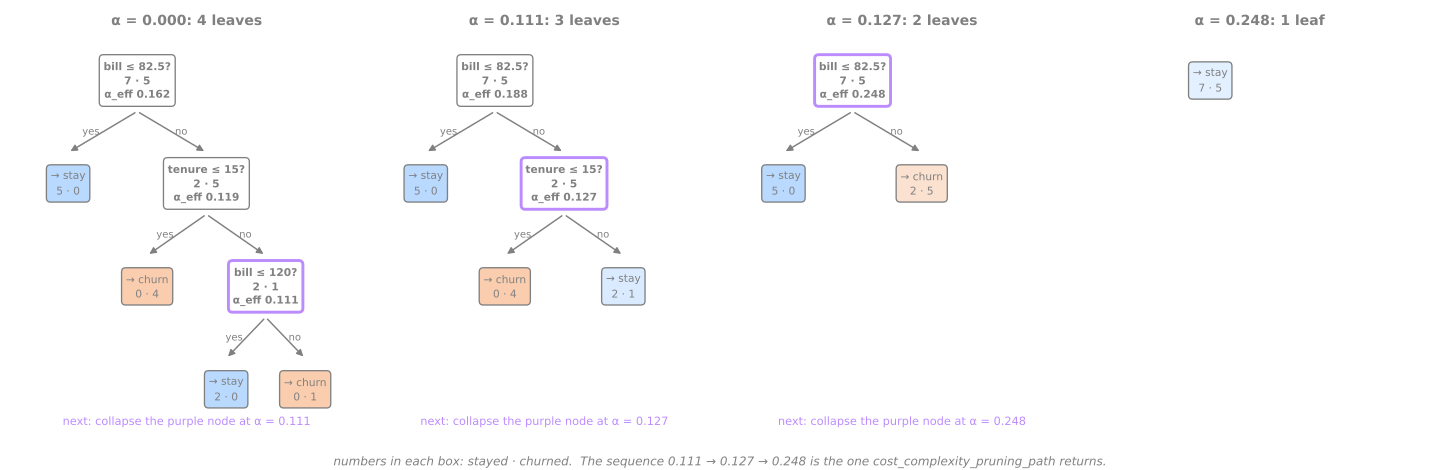
Qual \(\alpha\) usar é uma questão de hiperparâmetro, respondida por validação cruzada. No Spambase, o caminho da árvore completa tem mais de cem pontos de quebra; uma grade logarítmica de 22 valores o cobre:
from sklearn.model_selection import GridSearchCV

path = DecisionTreeClassifier(random_state=0).cost_complexity_pruning_path(X_dev, y_dev)
print(f"{len(path.ccp_alphas)} breakpoints, from {path.ccp_alphas[1]:.5f} to {path.ccp_alphas[-1]:.4f}")

alphas = np.r_[0, np.geomspace(1e-4, 1e-2, 21)]
search = GridSearchCV(DecisionTreeClassifier(random_state=0), {'ccp_alpha': alphas}, cv=cv)
search.fit(X_dev, y_dev)
res = pd.DataFrame({'ccp_alpha': alphas,
                    'leaves': [DecisionTreeClassifier(random_state=0, ccp_alpha=a).fit(X_dev, y_dev).get_n_leaves()
                               for a in alphas],
                    'validation': search.cv_results_['mean_test_score'],
                    'std': search.cv_results_['std_test_score']})
print(res.iloc[::2].round(5).to_string(index=False))

b = search.best_index_
se = res.loc[b, 'std'] / np.sqrt(5)                     # erro padrão da melhor média
simplest = res[res['validation'] >= res.loc[b, 'validation'] - se]['leaves'].idxmin()
for name, i in [('best', b), ('1-SE rule', simplest)]:
    print(f"{name:9s}: ccp_alpha {res.loc[i, 'ccp_alpha']:.5f} · {res.loc[i, 'leaves']} leaves · "
          f"validation {res.loc[i, 'validation']:.3f}")
122 breakpoints, from 0.00008 to 0.1479
 ccp_alpha  leaves  validation     std
   0.00000     221     0.90650 0.00845
   0.00013     213     0.90650 0.00845
   0.00020     213     0.90681 0.00847
   0.00032     160     0.90745 0.00877
   0.00050     109     0.91537 0.00767
   0.00079      68     0.91442 0.00567
   0.00126      40     0.90777 0.00811
   0.00200      26     0.90365 0.00779
   0.00316      15     0.89540 0.00961
   0.00501       8     0.89128 0.00741
   0.00794       7     0.89287 0.00706
best     : ccp_alpha 0.00050 · 109 leaves · validation 0.915
1-SE rule: ccp_alpha 0.00100 · 57 leaves · validation 0.913
(A tabela imprime uma linha a cada duas da grade; as contagens de folhas são as da árvore podada em todo o X_dev.) Podar de 221 para 109 folhas eleva a acurácia de validação de 0,906 para 0,915; abaixo de umas 40 folhas ela começa a cair, até 0,891 com 8 folhas. A regra de um erro padrão da aula de validação, que vem justamente deste livro (Breiman et al., 1984), fica com a árvore mais simples cujo escore está a menos de um erro padrão do melhor: 57 folhas com 0,913, um quarto da árvore completa, por uma perda que os folds não conseguem distinguir de zero. A figura mostra as duas famílias de remédios lado a lado (script da figura):
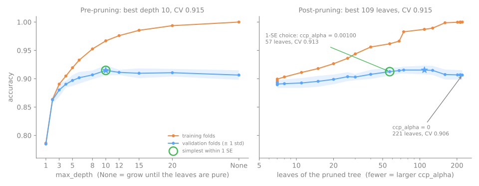
Os dois painéis têm a mesma forma da curva de C da regressão logística e da curva de k do k-NN: a acurácia de treino sobe com a complexidade, a de validação sobe, se achata e cai devagar. A poda não compra muita acurácia aqui (de 0,906 para 0,915). Seu maior trunfo é o tamanho: uma árvore com um quarto do tamanho, igualmente acurada e muito mais fácil de ler.
11. Instabilidade: uma pequena mudança, outra árvore
Etapa 3. Uma árvore é construída por uma cascata de escolhas, cada uma feita com os dados que chegaram àquele nó. Mude algumas linhas e a raiz pode escolher outro atributo ou outro limiar; tudo abaixo dela muda junto. Para medir isso, reajuste a árvore completa em 50 reamostras bootstrap do conjunto de desenvolvimento (tantas linhas quanto o original, sorteadas com reposição, de modo que cada reamostra deixa de fora cerca de um terço das linhas e repete outras) e compare as 50 árvores nos mesmos e-mails de teste:
rng = np.random.default_rng(0)
roots, preds = [], []
for b in range(50):
    idx = rng.integers(0, len(X_dev), len(X_dev))            # uma reamostra bootstrap
    m = DecisionTreeClassifier(random_state=0).fit(X_dev.iloc[idx], y_dev.iloc[idx])
    roots.append((X.columns[m.tree_.feature[0]], m.tree_.threshold[0], m.get_n_leaves()))
    preds.append(m.predict(X_test))
preds = np.array(preds)
roots = pd.DataFrame(roots, columns=['root feature', 'threshold', 'leaves'])
print(roots.groupby('root feature')['threshold'].agg(['count', 'min', 'max']).round(3))
print(f"leaves: from {roots['leaves'].min()} to {roots['leaves'].max()}")

acc = (preds == y_test.to_numpy()).mean(axis=1)
disagree = np.mean([np.mean(preds[i] != preds[j]) for i in range(50) for j in range(i + 1, 50)])
print(f"accuracy of each tree on the test rows: {acc.mean():.3f} (from {acc.min():.3f} to {acc.max():.3f})")
print(f"two trees disagree on {disagree:.1%} of the test e-mails")
print(f"majority vote of the 50 trees: {np.mean((preds.mean(axis=0) > 0.5) == y_test.to_numpy()):.3f}")
                  count    min    max
root feature
char_freq_!          19  0.067  0.150
char_freq_$          29  0.039  0.058
word_freq_free        1  0.015  0.015
word_freq_remove      1  0.010  0.010
leaves: from 136 to 186
accuracy of each tree on the test rows: 0.895 (from 0.873 to 0.919)
two trees disagree on 11.8% of the test e-mails
majority vote of the 50 trees: 0.950
A própria pergunta da raiz muda: char_freq_$ em 29 das 50 árvores, char_freq_! em 19 e duas outras palavras uma vez cada; o limiar de cada atributo também se move. As árvores têm entre 136 e 186 folhas. As acurácias são parecidas, 0,895 em média; o que muda é quais e-mails cada uma erra: duas árvores discordam em 11,8% dos e-mails de teste, quase tanto quanto cada uma delas erra. É isso que alta variância significa na prática. O mesmo acontece em duas dimensões, onde dá para ver (script da figura):
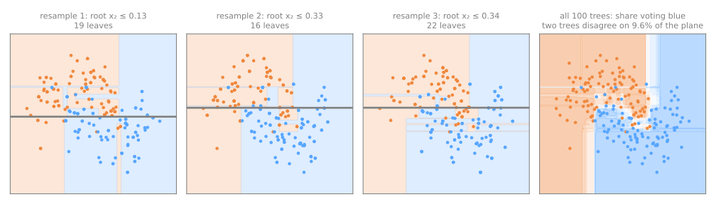
A última linha da saída é uma prévia. Cada árvore sozinha é pouco confiável, mas seus erros são em parte independentes, então deixar as 50 árvores votarem dá 0,950, melhor que a melhor árvore individual (0,919). Tirar a média de muitas árvores ajustadas em reamostras bootstrap se chama bagging; acrescentar aleatoriedade nos atributos que cada corte pode considerar o transforma na random forest, o assunto da próxima aula. A instabilidade é o defeito de uma árvore e a matéria-prima do ensemble.
12. O que as árvores dispensam e onde elas sofrem
Sem escalonamento
Etapa 4. Um corte x ≤ t só usa a ordem dos valores de um atributo. Qualquer transformação estritamente crescente de um atributo preserva essa ordem, então a árvore pode encontrar a mesma partição. Medido no Spambase:
from sklearn.preprocessing import StandardScaler

base = DecisionTreeClassifier(random_state=0).fit(X_dev, y_dev)
scaler = StandardScaler().fit(X_dev)
scaled = DecisionTreeClassifier(random_state=0).fit(scaler.transform(X_dev), y_dev)
logged = DecisionTreeClassifier(random_state=0).fit(np.log1p(X_dev), y_dev)

p = base.predict(X_test)
print(f"standardized: same prediction on {np.mean(scaled.predict(scaler.transform(X_test)) == p):.1%} of test rows")
print(f"log1p:        same prediction on {np.mean(logged.predict(np.log1p(X_test)) == p):.1%} of test rows, "
      f"{np.mean(logged.predict(np.log1p(X_dev)) == base.predict(X_dev)):.1%} of training rows")
print(f"test accuracy: raw {base.score(X_test, y_test):.3f} · standardized "
      f"{scaled.score(scaler.transform(X_test), y_test):.3f} · log1p {logged.score(np.log1p(X_test), y_test):.3f}")
standardized: same prediction on 100.0% of test rows
log1p:        same prediction on 99.3% of test rows, 100.0% of training rows
test accuracy: raw 0.923 · standardized 0.923 · log1p 0.922
Padronizar é uma transformação linear e não muda nada: as mesmas previsões em 100% das linhas de teste. O logaritmo também não muda a ordem de nada e as previsões de treino são idênticas; ainda assim, 0,7% das previsões de teste diferem. A razão é o ponto médio. Entre dois valores de treino vizinhos \(a < b\), a árvore original põe o limiar em \((a+b)/2\); a árvore com log o põe no ponto médio entre \(\log(1+a)\) e \(\log(1+b)\), que na escala original é \(\sqrt{(1+a)(1+b)} - 1\), um pouco abaixo de \((a+b)/2\). Um valor novo que caia entre esses dois limiares vai para a esquerda numa árvore e para a direita na outra. A partição das linhas de treino é idêntica; só a terra de ninguém entre elas se move. Portanto, escalonamento nunca é necessário; uma transformação monótona muda uma árvore só nas margens, enquanto pode mudar completamente um modelo linear ou um k-NN. Por isso as árvores são a escolha habitual para dados tabulares bagunçados, com colunas assimétricas e de cauda pesada, como rendas ou contagens.
Interações de graça
A árvore de churn usou tenure só dentro do ramo de conta alta: uma interação, "o tempo de casa importa quando a conta é alta". A regressão logística precisaria que você criasse à mão o produto tenure × bill ou um atributo parecido; uma árvore descobre efeitos condicionais assim aninhando perguntas. É uma das razões pelas quais as árvores e seus ensembles vão tão bem em dados tabulares nos quais ninguém sabe de antemão quais combinações importam.
Fronteiras diagonais viram escadas
O outro lado de cortar um atributo de cada vez: uma fronteira que depende de uma combinação de atributos, como \(x_2 > x_1\), só pode ser aproximada por muitos degraus alinhados aos eixos (script da figura):
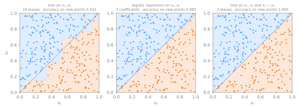
A árvore precisa de 16 folhas para o que a regressão logística diz com uma reta e, ainda assim, é pior em pontos novos (0,932 contra 0,985), porque os degraus ficam onde os 300 pontos de treino por acaso caíram. Dê à árvore o atributo \(x_2 - x_1\) e um único corte resolve o problema perfeitamente. Engenharia de atributos que expõe a combinação certa ajuda uma árvore mais do que qualquer hiperparâmetro.
Atributos categóricos e valores faltantes
Atributos categóricos. Em princípio, uma árvore pode dividir um atributo categórico diretamente: o CART manda um subconjunto das categorias para cada lado; o C4.5 abre um ramo por categoria. O DecisionTreeClassifier do scikit-learn (versão 1.9 no momento em que este texto foi escrito) só aceita números, então as categorias precisam ser codificadas: one-hot (uma coluna 0/1 por categoria; cada corte pergunta "é esta categoria?") ou códigos ordinais (1, 2, 3...), que impõem uma ordem arbitrária que a árvore ainda consegue desfazer com vários cortes. One-hot é o padrão seguro para um punhado de categorias; a aula de pré-processamento cobre os dois. O gradient boosting baseado em histogramas do scikit-learn e o LightGBM tratam categorias nativamente (gradient boosting).
Valores faltantes. Desde o scikit-learn 1.3, as árvores aceitam NaN diretamente. Quando um atributo tem valores faltantes num nó, o divisor avalia cada limiar duas vezes (uma mandando as linhas faltantes para a esquerda, outra para a direita) e fica com a melhor opção; na previsão, um valor faltante segue a direção aprendida para aquele nó. Na tabela de churn com duas contas apagadas:
gaps = customers.copy()
gaps.loc[['B', 'H'], 'bill'] = np.nan                      # duas contas nunca registradas
tree_nan = DecisionTreeClassifier(max_depth=2, random_state=0).fit(gaps[['tenure', 'bill']], y_c)
print(export_text(tree_nan, feature_names=['tenure', 'bill'], show_weights=True))
print("at the root, an unknown bill goes", "left" if tree_nan.tree_.missing_go_to_left[0] else "right")
print(tree_nan.predict_proba(pd.DataFrame({'tenure': [4, 40], 'bill': [np.nan, np.nan]})).round(3))
|--- bill <= 82.50
|   |--- weights: [5.00, 0.00] class: 0
|--- bill >  82.50
|   |--- tenure <= 15.00
|   |   |--- weights: [0.00, 4.00] class: 1
|   |--- tenure >  15.00
|   |   |--- weights: [2.00, 1.00] class: 0

at the root, an unknown bill goes right
[[0.    1.   ]
 [0.667 0.333]]
A árvore é a mesma que com os dados completos. Os clientes B (que cancelou) e H (que ficou) não têm conta. Mandá-los para o lado das contas altas mantém pura a folha das contas baixas, então foi isso que o divisor escolheu: "conta desconhecida" é tratada como "conta alta". Um cliente novo com conta desconhecida é então decidido pelo tempo de casa. Nenhum imputador é necessário; a regressão logística e o k-NN, ao contrário, falham com NaN e precisam de um no pipeline (você verá os dois no lab).
13. Importância de atributos e seu viés
Para cada atributo, feature_importances_ soma a queda de impureza de todos os cortes que o usam (ponderada pela fração das linhas de treino que chega a cada corte) e normaliza o resultado para somar 1. É de graça e muitas vezes útil, mas enviesada. Para ver como, acrescente ao Spambase duas colunas de puro ruído (uma contínua e uma binária) e cresça uma árvore completa:
noisy = X_dev.assign(random_number=rng.normal(size=len(X_dev)),          # ruído contínuo
                     random_coin=rng.integers(0, 2, len(X_dev)))          # ruído binário
deep = DecisionTreeClassifier(random_state=0).fit(noisy, y_dev)
imp = pd.Series(deep.feature_importances_, index=noisy.columns).sort_values(ascending=False)
print(imp.head(5).round(3).to_string())
for col in ['random_number', 'random_coin']:
    print(f"{col}: importance {imp[col]:.3f}, rank {list(imp.index).index(col) + 1} of {len(imp)}")
char_freq_$         0.311
word_freq_remove    0.161
char_freq_!         0.087
word_freq_hp        0.064
word_freq_free      0.039
random_number: importance 0.016, rank 12 of 59
random_coin: importance 0.002, rank 41 of 59
O topo da lista faz sentido: $, remove, !, hp, free. Mas uma coluna de números aleatórios, que por construção não carrega informação nenhuma, fica em 12º lugar entre 59, à frente de 46 atributos reais, enquanto a moeda aleatória fica em 41º. O mecanismo: no fundo da árvore, os nós são pequenos e ruidosos; um atributo contínuo com milhares de valores distintos oferece milhares de limiares, um dos quais vai separar algumas linhas ruidosas por acaso. Um atributo binário oferece um único limiar. A importância por impureza é calculada nos dados de treino, então recompensa essa memorização; ela é enviesada a favor de atributos com muitos valores distintos (Strobl et al., 2007). A solução é medir a importância em dados separados, embaralhando um atributo de cada vez e observando a queda do escore, a importância por permutação, que a próxima aula apresenta e Explicabilidade aprofunda, junto com o SHAP.
14. Perfil prático
| Como prevê | uma sequência de perguntas atributo ≤ limiar; a classe majoritária (ou a média) da folha, com as proporções de classe da folha como probabilidades |
| Como aprende | guloso, recursivo: em cada nó, o corte com a maior queda de impureza (Gini, entropia; MSE na regressão) |
| Hiperparâmetros | max_depth, min_samples_leaf, max_leaf_nodes, ccp_alpha, todos ajustados por validação cruzada |
| Pontos fortes | regras legíveis; sem escalonamento; transformações monótonas quase não importam; interações e não linearidade encontradas automaticamente; aceita NaN (scikit-learn ≥ 1.3); rápida para treinar e prever |
| Pontos fracos | sobreajusta se não for podada; instável (alta variância); escadas alinhadas aos eixos para fronteiras diagonais; regressão em escada que não extrapola; importância por impureza enviesada a favor de atributos com muitos valores; probabilidades grosseiras |
| Use quando | o modelo precisa ser lido, auditado ou aplicado à mão; caso contrário, use seus ensembles, random forests e gradient boosting |
Uma árvore, raramente; muitas árvores, o tempo todo
Uma árvore sozinha troca acurácia por legibilidade; na maioria dos problemas, a troca sai cara. Sua importância real está no papel de bloco de construção das random forests (muitas árvores profundas, com média, para cancelar a variância medida acima) e do gradient boosting (muitas árvores rasas, somadas uma após a outra, para reduzir o viés). Tudo o que está nesta aula — cortes, impureza, profundidade, tamanho de folha, poda — reaparece como hiperparâmetro desses dois.
Lab avançado — a chave final e o que ela vale
O lab fundamental terminou com uma chave de profundidade 2 que se lê bem (0,938) e uma árvore completa que acerta mais (0,969) mas não cabe num cartão. Esta parte procura a menor chave que não perde para a completa, compara-a com modelos que ninguém consegue ler, testa uma vez e mede o quanto as perguntas da chave dependem da amostra. Continue no mesmo notebook, na mesma sessão: os passos abaixo usam X, X_train, y_train, cv e cv_report dos passos 1 a 5.
Como fazer este lab em aula (cerca de 35 min, em duplas)
- Continue no notebook do Colab, a partir do passo 6. Se a sessão caiu, rode antes as células dos passos 1 a 5 (Ambiente de execução → Executar anteriores).
- Como no lab fundamental: Preveja antes de rodar, compare com esta página e tente as Simulações antes de abrir a solução.
- Ritmo sugerido: passos 6 e 7 e a primeira simulação em 15 min; passos 8 e 9 em 10 min; passo 10 e a segunda simulação em 10 min.
Passo 6 — ajustar profundidade, tamanho de folha e poda juntos
Preveja. Numa grade de 96 configurações, você espera um vencedor isolado ou várias configurações empatadas dentro do ruído dos folds? Qual delas caberia num cartão?
from sklearn.model_selection import GridSearchCV

grid = {'max_depth': [1, 2, 3, 4, 5, None],
        'min_samples_leaf': [1, 2, 5, 10],
        'ccp_alpha': [0, 0.01, 0.02, 0.05]}
search = GridSearchCV(DecisionTreeClassifier(random_state=0), grid, cv=cv)
search.fit(X_train, y_train)

res = pd.DataFrame(search.cv_results_['params'])
res['validation'] = search.cv_results_['mean_test_score']
res['std'] = search.cv_results_['std_test_score']
res['leaves'] = [DecisionTreeClassifier(random_state=0, **p).fit(X_train, y_train).get_n_leaves()
                 for p in search.cv_results_['params']]
print(f"{len(res)} configurations · best {search.best_params_} · {search.best_score_:.3f}")

sd = res.loc[search.best_index_, 'std']                   # desvio padrão entre folds do melhor
close = res[res['validation'] >= search.best_score_ - sd]
print(f"within one std ({sd:.3f}) of the best: {len(close)} configurations")
print(close.sort_values(['leaves', 'validation'], ascending=[True, False]).head(6).round(3).to_string())
96 configurations · best {'ccp_alpha': 0, 'max_depth': 4, 'min_samples_leaf': 1} · 0.969
within one std (0.009) of the best: 14 configurations
    ccp_alpha  max_depth  min_samples_leaf  validation    std  leaves
32       0.01        3.0                 1       0.961  0.025       6
33       0.01        3.0                 2       0.961  0.025       6
9        0.00        3.0                 2       0.961  0.025       7
36       0.01        4.0                 1       0.961  0.025       8
37       0.01        4.0                 2       0.961  0.025       8
40       0.01        5.0                 1       0.961  0.025       8
A melhor das 96 configurações é max_depth=4 com 0,969, o mesmo escore da árvore crescida até o fim, com 11 folhas. Os folds não conseguem separá-la das vizinhas: 14 configurações estão a menos de um desvio padrão entre folds (0,009) dela. A regra que escrevemos antes de olhar: a chave é a configuração com menos folhas a menos de um desvio padrão da melhor, a faixa mais folgada usada no lab da aula de validação (a faixa de um erro padrão, 0,004 aqui, só admite profundidade 4 ou mais, nenhuma do tamanho de um cartão). A vencedora é max_depth=3 com ccp_alpha=0.01: 6 folhas com 0,961. O parâmetro de poda faz o trabalho aqui: ele remove um corte que não se pagava (a árvore de profundidade 3 sem poda, na terceira linha, tem 7 folhas para o mesmo escore).
Passo 7 — os rivais, nos mesmos folds
Preveja. A regressão logística traça fronteiras retas em qualquer direção; a árvore, só degraus paralelos aos eixos. Sabendo que Adelie e Chinstrap diferem sobretudo na razão entre o comprimento e a profundidade do bico, quem você espera que vença?
from sklearn.impute import SimpleImputer
from sklearn.linear_model import LogisticRegression
from sklearn.neighbors import KNeighborsClassifier
from sklearn.pipeline import make_pipeline
from sklearn.preprocessing import StandardScaler

chosen = close.sort_values(['leaves', 'validation'], ascending=[True, False]).iloc[0]
params = {'max_depth': None if pd.isna(chosen['max_depth']) else int(chosen['max_depth']),
          'min_samples_leaf': int(chosen['min_samples_leaf']), 'ccp_alpha': float(chosen['ccp_alpha'])}
key = DecisionTreeClassifier(random_state=0, **params)
print("chosen tree:", params)

prep = lambda: [SimpleImputer(strategy='most_frequent'), StandardScaler()]   # estes modelos precisam dos dois
rivals = {
    'logistic': GridSearchCV(make_pipeline(*prep(), LogisticRegression(max_iter=5000)),
                             {'logisticregression__C': [0.01, 0.1, 1, 10, 100]}, cv=cv),
    'k-NN': GridSearchCV(make_pipeline(*prep(), KNeighborsClassifier()),
                         {'kneighborsclassifier__n_neighbors': [1, 3, 5, 9, 15, 25]}, cv=cv),
}
folds = pd.DataFrame({'tree': cross_validate(key, X_train, y_train, cv=cv)['test_score']})
for name, s in rivals.items():
    s.fit(X_train, y_train)
    print(f"{name}: {s.best_params_}")
    folds[name] = [s.cv_results_[f'split{k}_test_score'][s.best_index_] for k in range(5)]
folds['logistic - tree'] = folds['logistic'] - folds['tree']
folds['k-NN - tree'] = folds['k-NN'] - folds['tree']
print(folds.round(3).to_string())
print(pd.DataFrame({'mean': folds.mean(), 'std': folds.std(ddof=0)}).T.round(3).to_string())
chosen tree: {'max_depth': 3, 'min_samples_leaf': 1, 'ccp_alpha': 0.01}
logistic: {'logisticregression__C': 1}
k-NN: {'kneighborsclassifier__n_neighbors': 1}
    tree  logistic   k-NN  logistic - tree  k-NN - tree
0  0.981      1.00  0.981            0.019        0.000
1  0.922      0.98  1.000            0.059        0.078
2  0.980      1.00  0.980            0.020        0.000
3  0.941      0.98  1.000            0.039        0.059
4  0.980      1.00  1.000            0.020        0.020
       tree  logistic   k-NN  logistic - tree  k-NN - tree
mean  0.961     0.992  0.992            0.031        0.031
std   0.025     0.010  0.010            0.016        0.032
Os dois rivais precisam dos dois passos de pré-processamento que a árvore dispensou: um imputador para os sexos desconhecidos (com NaN eles falhariam) e um escalonador (sua penalização e suas distâncias dependem das unidades). Cada um é ajustado nos mesmos folds e a comparação é feita fold a fold, como na aula de validação:
- a regressão logística ajustada (\(C = 1\)) e o 1-NN ajustado chegam ambos a 0,992, contra 0,961 da chave;
- a regressão logística está à frente da chave nos cinco folds, por 0,031 ± 0,016 em média. A diferença média é cerca do dobro da sua dispersão: pela regra da aula de validação, uma diferença real, não um empate;
- o k-NN também está à frente na média, mas empata com a chave em dois folds (0,031 ± 0,032): no limite do ruído.
Por que um modelo linear vence a árvore? Volte ao passo 4: Adelie e Chinstrap diferem principalmente na razão entre comprimento e profundidade do bico, uma fronteira diagonal no plano desses dois atributos. A árvore a aproxima com uma escada, exatamente como na figura da escada; a regressão logística a traça diretamente. Então a legibilidade custa cerca de 3 pontos de acurácia neste problema. A equipe de campo pediu uma chave, então é a chave que vai para o teste; se só a acurácia importasse, a regra mandaria a regressão logística em seu lugar. Só uma das duas pode ser testada.
Simulação: dê a diagonal à árvore. O passo 7 atribuiu a derrota da chave a uma fronteira diagonal entre Adelie e Chinstrap. Teste a explicação: acrescente a razão culmen_length_mm / culmen_depth_mm como coluna e refaça a validação cruzada da mesma receita (profundidade 3, ccp_alpha=0.01). A acurácia sobe? A razão vira a raiz? Quantas folhas a chave precisa agora?
Solução
Xr = X.assign(bill_ratio=X['culmen_length_mm'] / X['culmen_depth_mm'])    # o atributo diagonal
Xr_train = Xr.loc[X_train.index]                                           # as mesmas linhas de treino
r = cross_validate(DecisionTreeClassifier(random_state=0, **params), Xr_train, y_train, cv=cv,
                   return_estimator=True)
print(f"key with bill_ratio: validation {r['test_score'].mean():.3f} ± {r['test_score'].std():.3f}")
m = DecisionTreeClassifier(random_state=0, **params).fit(Xr_train, y_train)
print(f"leaves {m.get_n_leaves()} · root: {Xr.columns[m.tree_.feature[0]]} <= {m.tree_.threshold[0]:.2f}")
print(export_text(m, feature_names=list(Xr.columns), show_weights=True))
key with bill_ratio: validation 0.973 ± 0.020
leaves 5 · root: bill_ratio <= 2.45
|--- bill_ratio <= 2.45
|   |--- culmen_length_mm <= 43.35
|   |   |--- weights: [108.00, 0.00, 0.00] class: Adelie
|   |--- culmen_length_mm >  43.35
|   |   |--- is_male <= 0.50
|   |   |   |--- weights: [0.00, 4.00, 0.00] class: Chinstrap
|   |   |--- is_male >  0.50
|   |   |   |--- weights: [5.00, 0.00, 0.00] class: Adelie
|--- bill_ratio >  2.45
|   |--- island_Biscoe <= 0.50
|   |   |--- weights: [0.00, 47.00, 0.00] class: Chinstrap
|   |--- island_Biscoe >  0.50
|   |   |--- weights: [0.00, 0.00, 92.00] class: Gentoo
A razão vira a raiz (bill_ratio <= 2.45) e a chave sobe de 0,961 para 0,973 ± 0,020, com 5 folhas em vez de 6: um único atributo construído fez mais que a grade inteira do passo 6 e a distância para a regressão logística cai de 0,031 para 0,019. A chave nova também se lê de outro jeito: bico comprido e fino (razão acima de 2,45) é Chinstrap ou Gentoo, separados pela ilha. Leia as folhas com cuidado, porém: a separação Chinstrap/Gentoo usa de novo a ilha (um fato sobre onde as aves foram medidas, não sobre a espécie) e duas folhas se apoiam em 4 e 5 aves, decididas pelo sexo. É a figura da escada em dados reais: a combinação certa de atributos vale mais que qualquer hiperparâmetro.
Passo 8 — o único teste
Preveja. A validação cruzada deu 0,961 ± 0,025 para a chave. No teste, você espera um resultado parecido? Que par de espécies deve concentrar os erros?
from sklearn.metrics import confusion_matrix

key.fit(X_train, y_train)
pred = key.predict(X_test)
print(f"test accuracy {np.mean(pred == y_test):.3f} · misidentified: {np.sum(pred != y_test)} of {len(y_test)}")
print(pd.DataFrame(confusion_matrix(y_test, pred), index=key.classes_, columns=key.classes_))
test accuracy 0.988 · misidentified: 1 of 86
           Adelie  Chinstrap  Gentoo
Adelie         38          0       0
Chinstrap       1         16       0
Gentoo          0          0      31
A chave, reajustada nos 256 pinguins de desenvolvimento, encontra os 86 pinguins de teste uma vez: 0,988, um erro, um Chinstrap identificado como Adelie, o par com que a chave tem dificuldade. Isso fica acima da estimativa da CV de 0,961 ± 0,025, por cerca de um desvio padrão; com um erro valendo 1,2 ponto, o conjunto de teste também é uma medida ruidosa. A matriz de confusão mostra que o Gentoo nunca é confundido com nada: a pergunta "nadadeira longa e bico raso?" o isola por completo.
Passo 9 — a chave e o que ela usa
Preveja. Das 8 colunas, quais você espera ver na chave? Alguma delas pode estar ali por um motivo que não tem nada a ver com biologia?
print(export_text(key, feature_names=list(X.columns), show_weights=True))
imp = pd.Series(key.feature_importances_, index=X.columns)
print(imp[imp > 0].sort_values(ascending=False).round(3).to_string())
|--- flipper_length_mm <= 206.50
|   |--- culmen_length_mm <= 43.35
|   |   |--- weights: [107.00, 4.00, 0.00] class: Adelie
|   |--- culmen_length_mm >  43.35
|   |   |--- island_Dream <= 0.50
|   |   |   |--- weights: [3.00, 0.00, 1.00] class: Adelie
|   |   |--- island_Dream >  0.50
|   |   |   |--- weights: [1.00, 42.00, 0.00] class: Chinstrap
|--- flipper_length_mm >  206.50
|   |--- culmen_depth_mm <= 17.55
|   |   |--- weights: [0.00, 0.00, 91.00] class: Gentoo
|   |--- culmen_depth_mm >  17.55
|   |   |--- culmen_depth_mm <= 18.95
|   |   |   |--- weights: [2.00, 0.00, 0.00] class: Adelie
|   |   |--- culmen_depth_mm >  18.95
|   |   |   |--- weights: [0.00, 5.00, 0.00] class: Chinstrap

flipper_length_mm    0.548
culmen_length_mm     0.328
culmen_depth_mm      0.087
island_Dream         0.037
A chave impressa tem 6 folhas e pode ser lida em voz alta:
- nadadeira ≤ 206,5 mm e comprimento do bico ≤ 43,35 mm → Adelie (107 de 111);
- nadadeira ≤ 206,5 mm, comprimento do bico > 43,35 mm, fora da ilha Dream → Adelie (3 de 4);
- nadadeira ≤ 206,5 mm, comprimento do bico > 43,35 mm, na ilha Dream → Chinstrap (42 de 43);
- nadadeira > 206,5 mm e profundidade do bico ≤ 17,55 mm → Gentoo (91 de 91);
- nadadeira > 206,5 mm e 17,55 < profundidade do bico ≤ 18,95 mm → Adelie (2 de 2);
- nadadeira > 206,5 mm e profundidade do bico > 18,95 mm → Chinstrap (5 de 5).
A mesma chave desenhada como um cartão de campo (script da figura):
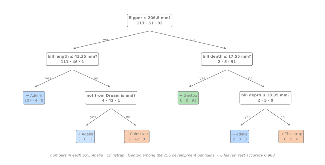
A regra 3 usa a ilha: neste conjunto, os Chinstraps só foram amostrados em Dream, então "bico longo em Dream" é uma pista forte. É um fato sobre onde essas aves foram medidas, não sobre a espécie. Um biólogo lendo a chave apontaria isso; um modelo que ninguém lê o usaria em silêncio. As regras 5 e 6 se apoiam em 2 e 5 aves, o tipo de folha que a regra de poda tolerou mas que merece pouca confiança. As importâncias confirmam a leitura: comprimento da nadadeira (0,548) e comprimento do bico (0,328) carregam a chave; massa corporal e sexo nunca são usados. Lembre-se do viés medido acima; com 256 linhas e 5 cortes, essas importâncias dizem "quais perguntas a chave faz" e nada além disso.
Passo 10 — quão estável é a chave?
Preveja. Se outra equipe medisse pinguins parecidos e rodasse a mesma receita, a chave começaria pela mesma pergunta? E as previsões, mudariam tanto quanto as perguntas?
rng = np.random.default_rng(0)
roots, preds = [], []
for b in range(100):
    idx = rng.integers(0, len(X_train), len(X_train))             # reamostra bootstrap
    m = DecisionTreeClassifier(random_state=0, **params).fit(X_train.iloc[idx], y_train.iloc[idx])
    roots.append((X.columns[m.tree_.feature[0]], round(m.tree_.threshold[0], 2)))
    preds.append(m.predict(X_test))
roots = pd.DataFrame(roots, columns=['feature', 'threshold'])
print(roots.groupby('feature')['threshold'].agg(['count', 'min', 'max']))
preds = np.array(preds)
disagree = np.mean([np.mean(preds[i] != preds[j]) for i in range(100) for j in range(i + 1, 100)])
print(f"two resampled keys disagree on {disagree:.1%} of the test penguins")
print(f"test penguins on which all 100 keys agree: {np.mean((preds == preds[0]).all(axis=0)):.1%}")
                   count     min     max
feature
culmen_depth_mm       12   16.05   16.40
culmen_length_mm      32   41.55   43.35
flipper_length_mm     56  202.50  207.50
two resampled keys disagree on 4.1% of the test penguins
test penguins on which all 100 keys agree: 73.3%
A mesma receita (profundidade 3, ccp_alpha=0.01) aplicada a 100 reamostras bootstrap do conjunto de desenvolvimento produz chaves que começam com três perguntas diferentes: comprimento da nadadeira em 56 delas, comprimento do bico em 32, profundidade do bico em 12. Impressas num cartão, pareceriam três chaves diferentes. Suas previsões diferem menos que sua estrutura, porque nas aves fáceis todas as chaves concordam: duas chaves discordam em 4,1% dos pinguins de teste e as 100 concordam em 73,3% deles. Eis o significado prático da instabilidade: as perguntas específicas de uma árvore não são uma descoberta sobre pinguins; são uma de várias maneiras igualmente boas de cortar esta amostra. Leia as regras como ferramenta de trabalho, não como biologia. E não se surpreenda se os dados da próxima temporada produzirem outra chave.
Simulação: bagging à mão. O passo 10 mostrou que chaves treinadas em reamostras diferentes discordam. Use isso a seu favor: dentro de cada fold do cv, ajuste 100 árvores crescidas até o fim, cada uma numa reamostra bootstrap do treino do fold, e deixe-as votar (a espécie mais frequente entre as 100 previsões). Compare com uma única árvore crescida até o fim, nos mesmos folds.
Solução
votes_acc, single_acc = [], []
for tr, va in cv.split(X_train, y_train):
    Xa, ya, Xv, yv = X_train.iloc[tr], y_train.iloc[tr], X_train.iloc[va], y_train.iloc[va]
    bag = np.random.default_rng(0)
    preds = []
    for b in range(100):
        idx = bag.integers(0, len(Xa), len(Xa))                    # uma reamostra bootstrap do fold
        preds.append(DecisionTreeClassifier(random_state=0).fit(Xa.iloc[idx], ya.iloc[idx]).predict(Xv))
    vote = pd.DataFrame(preds).mode(axis=0).iloc[0].to_numpy()     # a espécie mais votada
    votes_acc.append(np.mean(vote == yv.to_numpy()))
    single_acc.append(DecisionTreeClassifier(random_state=0).fit(Xa, ya).score(Xv, yv))
print(f"one fully grown tree: {np.mean(single_acc):.3f} ± {np.std(single_acc):.3f}")
print(f"vote of 100 trees:    {np.mean(votes_acc):.3f} ± {np.std(votes_acc):.3f}")
print("per fold, vote - single:", np.round(np.array(votes_acc) - np.array(single_acc), 3))
one fully grown tree: 0.969 ± 0.016
vote of 100 trees:    0.976 ± 0.019
per fold, vote - single: [0.019 0.02  0.    0.    0.   ]
O voto de 100 árvores marca 0,976, contra 0,969 de uma árvore só: ganha em dois folds, empata nos outros três e nunca perde. O ganho é pequeno porque, nos pinguins, uma árvore já erra pouco; o mecanismo é o mesmo do Spambase na seção 11 (de 0,895 para 0,950): os erros de árvores treinadas em reamostras diferentes são em parte independentes e o voto cancela uma parte deles. Você acabou de construir a maior parte de uma random forest; falta só sortear também os atributos que cada corte pode usar, o assunto da próxima aula.
Para fechar a aula. Em uma frase cada: (1) por que a chave perdeu para a regressão logística e o que a recuperou em parte? (2) Por que chaves treinadas em reamostras diferentes começam por perguntas diferentes? (3) Por que o voto de muitas árvores erra menos que uma árvore só?
Sua vez (avançado)
Para casa, com mais tempo:
- Entropia na grade. Acrescente
'criterion': ['gini', 'entropy']à grade do passo 6. Quantas das configurações a menos de um desvio padrão da melhor usam entropia? A chave escolhida muda? - Uma árvore de regressão. No CSV de imóveis da Califórnia (
pd.read_csv('https://raw.githubusercontent.com/hsandmann/biblio/refs/heads/main/ml/aula02/housing.csv')), prevejamedian_house_valuea partir das colunas numéricas com umDecisionTreeRegressor. Ajustemax_depthemin_samples_leafcomKFold(5, shuffle=True, random_state=0)e compare o RMSE da melhor árvore com o de umaLinearRegression. Qual é o maior valor que a árvore pode prever? Por quê? - Importância por permutação. Calcule
permutation_importance(key, X_test, y_test, n_repeats=30, random_state=0)(desklearn.inspection) e compare com as importâncias por impureza do passo 9. A ilha Dream continua importando? Algum atributo que a chave não usa ganha importância?
Referências
- Breiman, L.; Friedman, J. H.; Olshen, R. A.; Stone, C. J. Classification and Regression Trees. Wadsworth (1984) — o CART: cortes binários, Gini, árvores de regressão, poda por custo-complexidade e a regra de um erro padrão. DOI
- Quinlan, J. R. "Induction of Decision Trees." Machine Learning 1, n. 1 (1986): 81–106 — o ID3 e o ganho de informação. DOI
- Quinlan, J. R. C4.5: Programs for Machine Learning. Morgan Kaufmann (1993) — o sucessor do ID3, com razão de ganho, atributos contínuos, valores faltantes e poda.
- Morgan, J. N.; Sonquist, J. A. "Problems in the Analysis of Survey Data, and a Proposal." Journal of the American Statistical Association 58, n. 302 (1963): 415–434 — o AID, a primeira árvore de regressão. DOI
- Hyafil, L.; Rivest, R. L. "Constructing Optimal Binary Decision Trees is NP-Complete." Information Processing Letters 5, n. 1 (1976): 15–17 — por que todo algoritmo prático é guloso. DOI
- Raileanu, L. E.; Stoffel, K. "Theoretical Comparison between the Gini Index and Information Gain Criteria." Annals of Mathematics and Artificial Intelligence 41 (2004): 77–93 — os dois critérios discordam em cerca de 2% dos cortes. DOI
- Strobl, C.; Boulesteix, A.-L.; Zeileis, A.; Hothorn, T. "Bias in Random Forest Variable Importance Measures: Illustrations, Sources and a Solution." BMC Bioinformatics 8 (2007): 25 — a importância por impureza favorece atributos com muitos valores. DOI
- Hastie, T.; Tibshirani, R.; Friedman, J. The Elements of Statistical Learning. 2ª ed., Springer (2009), seção 9.2 — árvores, medidas de impureza, poda, instabilidade. PDF gratuito
- Hopkins, M.; Reeber, E.; Forman, G.; Suermondt, J. "Spambase." UCI Machine Learning Repository (1999) — os e-mails usados nesta aula (OpenML 44). DOI
- Gorman, K. B.; Williams, T. D.; Fraser, W. R. "Ecological Sexual Dimorphism and Environmental Variability within a Community of Antarctic Penguins (Genus Pygoscelis)." PLoS ONE 9, n. 3 (2014): e90081 — os pinguins do lab (OpenML 42585). DOI
Quiz
O quiz cobre a abordagem fundamental.