Gradiente Descendente & Regularização

A solução em forma fechada dos mínimos quadrados ordinários (OLS) é elegante, mas não escala para grandes quantidades de atributos, não existe para a maioria dos outros modelos e nada diz sobre controlar o sobreajuste. Esta aula acrescenta as duas ferramentas que fazem isso: o gradiente descendente — o motor de otimização por trás de quase todo o ML moderno — e a regularização — o freio padrão para a complexidade do modelo.

A aula deduz o gradiente para uma reta, dá os primeiros passos à mão em três pontos e depois deixa o código refazer cada um desses números. Ela mede como um polinômio flexível demais sobreajusta e mostra o que o ridge e o lasso fazem com os coeficientes, primeiro num único coeficiente que dá para acompanhar com um lápis, depois em muitos atributos de uma vez.

Como esta aula está organizada

A aula tem duas abordagens. Cada uma tem slides, texto e um lab para fazer em aula no Colab; o quiz do fim cobre a fundamental. Comece pela fundamental: a avançada parte dela.

Os dois labs usam o mesmo notebook no Colab: a parte fundamental são as suas seções 1 a 3; a avançada, as seções 4 a 6. Tudo roda no navegador; não é preciso baixar nada.

Abordagem fundamental

Uma pergunta guia esta parte: como um modelo acha seus pesos sem resolver uma equação e como impedir que um modelo flexível decore? A resposta para a primeira metade é uma regra, repetida: meça a inclinação, dê um passo contra ela. A resposta para a segunda metade é um termo a mais na perda. As duas são feitas primeiro à mão, em três pontos e num coeficiente, e depois conferidas no código.

Esta parte segue um caminho em quatro etapas, desenhado abaixo: 1. descer a ladeira; 2. ajustar o passo; 3. retas → curvas; 4. regularizar. Cada etapa leva à sua seção e, nos slides, uma faixa embaixo mostra em que etapa você está.

Slides da abordagem fundamental

Clique nos slides e use as setas ← → para navegar; F abre em tela cheia e Esc mostra todos os slides. Abrir os slides numa aba nova

1. Gradiente descendente

Etapa 1. A ideia é a que fecha a aula anterior. Para achar o mínimo de uma perda \(J(w)\), em vez de resolver \(\nabla J = 0\) no papel, desça a ladeira: meça a inclinação onde você está, dê um passo contra ela, repita.

O \(\eta\) é a taxa de aprendizado, o tamanho do passo. O gradiente \(\nabla_w J\) aponta para onde a perda mais cresce, então é o sinal de menos que faz o método descer em vez de subir.

Falta uma coisa só para isso virar código: saber o que é \(\nabla_w J\). Ele é uma lista de derivadas parciais, uma para cada parâmetro, que vale a pena montar à mão antes de aceitar a forma matricial pronta.

2. De onde vem o gradiente

A aula anterior esboçou esta conta para a reta de dois parâmetros; aqui ela é feita devagar, porque o mesmo padrão depois vale para qualquer número de parâmetros (seção 9, na parte avançada). Escreva a perda como média, para a escala não depender de \(n\):

Cada parcela é o quadrado de um resíduo, \(e_i^2\). Pela regra da cadeia, a derivada de \(e_i^2\) em relação a qualquer parâmetro é \(2e_i\) vezes a derivada de \(e_i\) em relação a esse parâmetro. Ou seja: tudo se reduz a saber como o resíduo reage a cada peso. E isso é simples, porque \(e_i\) depende dos pesos de forma linear:

O \(-1\) aparece porque subir o intercepto em uma unidade baixa todo resíduo em uma unidade. O \(-x_i\) aparece porque subir a inclinação em uma unidade baixa o resíduo em \(x_i\) — quanto mais longe o ponto está da origem, mais ele sente uma mudança de inclinação.

Substituindo:

Veja do que cada derivada é feita: uma soma de resíduos, cada um pesado pelo quanto o seu ponto sente o parâmetro. O ponto que a reta já acerta entra com \(e_i \approx 0\) e quase não vota; o ponto em que ela erra feio domina o passo.

Um passo, à mão

Três pontos — \((1,2), (2,4), (3,7)\) — partindo de \(w_0 = w_1 = 0\), com \(\eta = 0{,}1\).

Com os dois pesos zerados a reta prevê 0 em toda parte, então o resíduo é o próprio \(y\):

Aplique as duas fórmulas que acabamos de deduzir:

As duas deram negativas, o que faz sentido: os dois pesos estão baixos demais e aumentar qualquer um reduz a perda. O passo, então, aumenta os dois:

Só nesse passo a perda cai de \(J = 23\) para \(J = 0{,}625\). Repetindo o procedimento:

Leia a tabela devagar, porque ela mostra três coisas de uma vez.

O primeiro passo é enorme: a perda cai de 23 para 0,63, quase todo o trabalho. Depois o progresso se arrasta — 0,344, depois 0,327. Esse formato é a regra, não a exceção — é por isso que ver \(J\) cair rápido no início não diz quase nada sobre ter convergido.

Os gradientes trocam de sinal: os dois viram entre as iterações 0 e 1; \(\partial J/\partial w_1\) vira de novo na iteração 2. É um passo ultrapassando o mínimo e o seguinte voltando atrás — o mesmo vaivém que o simulador da taxa de aprendizado mostra adiante, aqui em escala pequena.

E os dois parâmetros não andam no mesmo ritmo: na iteração 0 a derivada em \(w_1\) é 2,4 vezes a de \(w_0\), porque cada resíduo entra na conta de \(w_1\) multiplicado por \(x_i\), que vale até 3. Guarde essa assimetria — ela é o assunto da paisagem, na parte avançada (seção 10).

Deixando rodar até 2000 iterações chega-se a \(w_0 = -0{,}667\) e \(w_1 = 2{,}5\), exatamente o que as equações normais dão — a mesma resposta, por um caminho mais lento.

O simulador refaz esta tabela uma iteração por vez: em cada passo ele mostra os resíduos da reta atual, as duas derivadas, a atualização e a perda antes e depois; também pode pular para a iteração 2000.

3. A taxa de aprendizado

Etapa 2. A regra tem um botão só, que decide tudo:

• \(\eta\) pequeno demais → passos minúsculos, convergência dolorosamente lenta;
• \(\eta\) grande demais → os passos ultrapassam o mínimo; a perda oscila ou diverge;
• receita prática: experimente \(\eta \in \{10^{-3}, 10^{-2}, 10^{-1}\}\), monitore a curva de perda de treino — ela deve cair suavemente.

Experimente você mesmo. Na perda abaixo o limiar fica exatamente em \(\eta = 1\), que põe a história inteira num lugar só: em \(\eta = 0{,}5\) o passo acerta o mínimo de uma vez; abaixo disso ele se aproxima aos poucos; entre 0,5 e 1 ele passa do ponto mas ainda fecha, pulando de um lado para o outro; em \(\eta = 1\) exatamente ele fica batendo entre os mesmos dois pontos para sempre, sem nunca chegar mais perto; acima de 1 ele explode. Defina \(\eta = 1{,}05\) e avance passo a passo:

Por que exatamente 1? A perda do simulador é uma parábola de curvatura 2, como \(J(w) = (w-3)^2\), cuja inclinação é \(2(w-3)\). Subtraia 3 dos dois lados da atualização e a distância até o mínimo fica multiplicada por \((1 - 2\eta)\) a cada passo: ela encolhe enquanto \(|1 - 2\eta| < 1\), ou seja, \(0 < \eta < 1\). O passo 2 do lab confere isso no código.

4. Batch, estocástico e mini-batch

A segunda escolha é quantos dados cada passo olha. O gradiente acima soma sobre os \(n\) pontos; com milhões de linhas, um passo custa uma passada pelo conjunto inteiro.

from sklearn.linear_model import SGDRegressor
model = SGDRegressor(loss='squared_error', penalty='l2', alpha=1e-4,
                     learning_rate='invscaling', max_iter=1000)

O mesmo laço — com perdas diferentes — treina a regressão logística, as SVMs e as redes neurais. Aprenda-o uma vez, reutilize em todo lugar. O passo 6 do lab avançado escreve o laço de mini-batch e o roda em 20.640 casas.

5. De retas a curvas: atributos polinomiais

Etapa 3. A regressão linear é linear nos parâmetros, não necessariamente nas entradas. Expandir os atributos para potências, \(x \mapsto (x, x^2, \dots, x^p)\), ajusta polinômios com a mesma maquinaria do OLS:

from sklearn.pipeline import make_pipeline
from sklearn.preprocessing import PolynomialFeatures

model = make_pipeline(PolynomialFeatures(degree=3), LinearRegression())

Mas a flexibilidade é uma faca de dois gumes:

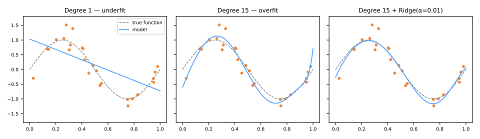
O grau 1 subajusta — rígido demais para seguir o seno. O grau 15 sobreajusta — 16 parâmetros perseguem 25 pontos ruidosos, produzindo oscilações violentas. O painel da direita mantém todos os 16 parâmetros mas adiciona uma penalidade Ridge: a curva relaxa de volta ao sinal. Isso é a regularização em ação.

Subajuste e sobreajuste, medidos

A figura convence o olho. Vale medir, porque o número mostra uma coisa que o desenho esconde.

Os dados são 100 pontos de \(y = 0{,}5x^2 + x + 2\) com ruído de desvio 3, para \(x\) entre \(-3\) e \(3\). Três modelos: grau 1, grau 2 — o grau certo — e grau 30. Para cada um, o erro no próprio treino ao lado do erro em validação cruzada de cinco dobras: os dados são cortados em cinco partes; o modelo treina em quatro e é avaliado na quinta, num rodízio que se repete até cada parte ter sido avaliada uma vez. As cinco notas dão uma média e um desvio; a técnica em si é o tema da aula de validação cruzada.

O grau 30 tem o menor erro de treino dos três. Quem escolhesse o modelo por essa coluna escolheria justamente o pior.

A coluna mais instrutiva, porém, é a última. Veja as cinco dobras do grau 30 uma a uma:

Em três das cinco ele vai tão bem quanto o grau 2. Em uma delas, explode. Sobreajuste não é errar sempre — é errar de forma imprevisível — é por isso que a variação entre dobras denuncia o problema antes da média denunciar.

Daí sai um diagnóstico de bolso:

Existe também um piso. O ruído tem desvio 3 e essa parcela do \(y\) não depende de \(x\), então nenhum modelo consegue removê-la. O grau 2 chega perto desse piso, que é tudo o que se pode pedir de um modelo.

Se um grau é "complexo demais" depende também de quantos pontos existem: a seção 11, na parte avançada, mede isso.

6. Regularização

Etapa 4. Em vez de restringir o número de parâmetros, penalize sua magnitude — adicione um termo de complexidade à perda:

Ridge (L2) — Tikhonov, 1943; Hoerl & Kennard, 1970

• encolhe todos os coeficientes suavemente em direção a zero (nunca exatamente zero);
• distribui o peso entre atributos correlacionados — a cura padrão para a multicolinearidade;
• a forma fechada ainda existe: \(\hat{w} = (X^\top X + \alpha I)^{-1} X^\top y\) — o \(\alpha I\) torna a matriz inversível mesmo com atributos colineares.

Lasso (L1) — Tibshirani, 1996

• a penalidade de valor absoluto tem quinas em zero: as soluções pousam exatamente em zero para atributos fracos;
• realiza seleção automática de atributos — os coeficientes não nulos que sobrevivem nomeiam os atributos que importam;
• entre um grupo de atributos altamente correlacionados, tende a manter um arbitrariamente e zerar o resto.

O Elastic Net mistura ambas as penalidades (l1_ratio) — um padrão robusto quando os atributos são muitos e correlacionados.

from sklearn.linear_model import Ridge, Lasso, ElasticNet

Ridge(alpha=1.0)
Lasso(alpha=0.1)
ElasticNet(alpha=0.1, l1_ratio=0.5)

O caso unidimensional, em forma fechada

Com um único atributo, escalonado para que \(\sum_i x_i^2 = 1\), as duas penalidades têm solução explícita; dá para deduzi-las em duas linhas. O coeficiente do OLS é \(\hat{w} = \sum_i x_i y_i\) e o erro quadrático é \(\sum_i (y_i - w x_i)^2 = \sum_i y_i^2 - 2w\hat{w} + w^2\). Some cada penalidade e iguale a derivada a zero:

A primeira dá uma divisão; a segunda, uma subtração, que só tem solução positiva enquanto \(\hat{w} > \alpha/2\) (fora disso o mínimo fica em \(w = 0\)):

Com \(\alpha = 1\):

O ridge divide; divisão nunca chega a zero. O lasso subtrai uma quantidade fixa e corta em zero — então todo coeficiente abaixo do limiar \(\alpha/2\) não encolhe, desaparece. Esse corte é a seleção automática de atributos das listas acima, escrita como fórmula; a seção 12 mostra a sua geometria.

O simulador preenche esta tabela uma linha por vez: o passo 0 deduz as duas fórmulas e cada passo seguinte divide e subtrai para uma linha da tabela, ao lado de um gráfico do coeficiente penalizado contra o do OLS.

7. O botão α

O \(\alpha\) troca fidelidade aos dados por tamanho dos coeficientes:

• \(\alpha \to 0\): OLS puro (sem freio);
• \(\alpha \to \infty\): todos os coeficientes esmagados para ~0, o modelo prevê a média (freio total);
• o \(\alpha\) certo não é conhecido de antemão — é escolhido por validação cruzada (RidgeCV, LassoCV ou uma busca em grade).

8. Resumo: o motor e o freio em cinco linhas

1. O gradiente descendente desce a ladeira: \(w \leftarrow w - \eta\,\nabla J\), com o gradiente medido onde você está.
2. No erro quadrático, o gradiente é uma soma ponderada pelos resíduos: \(-\frac{2}{n}\sum_i e_i\) para o intercepto, \(-\frac{2}{n}\sum_i e_i x_i\) para a inclinação.
3. A taxa de aprendizado decide o regime: pequena demais rasteja, grande demais diverge. Mini-batches deixam cada passo barato.
4. Modelos flexíveis sobreajustam: erro de treino baixo, erro de validação alto e imprevisível. A variação entre dobras denuncia.
5. A regularização penaliza o tamanho dos coeficientes: o ridge os divide, o lasso os subtrai e corta em zero; escalone antes e escolha \(\alpha\) por validação cruzada.

Lab fundamental — ladeira abaixo, um passo de cada vez

O problema. Até aqui tudo foi fórmula e tabela feitas à mão. Este lab escreve a regra de atualização em poucas linhas de numpy, quebra-a de propósito forçando a taxa de aprendizado e treina uma reta nos três pontos de um passo, à mão, conferindo cada número da tabela e a resposta final contra a forma fechada. Nenhuma biblioteca faz a descida por nós: a ideia é ver o laço.

Passo 1 — descer uma ladeira de uma variável

Preveja. A perda mais simples possível, \(J(w) = (w-3)^2\), partindo de \(w = 0\) com \(\eta = 0{,}1\) fixo. Os passos vão ter todos o mesmo tamanho? O \(w\) vai passar de 3 em algum momento?

import numpy as np
import matplotlib.pyplot as plt


def J(w):
    return (w - 3) ** 2          # a perda: mínimo em w = 3


def dJ(w):
    return 2 * (w - 3)           # a sua inclinação


w, eta = 0.0, 0.1                # palpite inicial e taxa de aprendizado
print(f"{'step':>4} {'w':>8} {'J(w)':>9} {'dJ/dw':>8}")
for step in range(11):
    print(f"{step:>4} {w:>8.4f} {J(w):>9.4f} {dJ(w):>8.4f}")
    w = w - eta * dJ(w)

step        w      J(w)    dJ/dw
   0   0.0000    9.0000  -6.0000
   1   0.6000    5.7600  -4.8000
   2   1.0800    3.6864  -3.8400
   3   1.4640    2.3593  -3.0720
   4   1.7712    1.5099  -2.4576
   5   2.0170    0.9664  -1.9661
   6   2.2136    0.6185  -1.5729
   7   2.3709    0.3958  -1.2583
   8   2.4967    0.2533  -1.0066
   9   2.5973    0.1621  -0.8053
  10   2.6779    0.1038  -0.6442

A taxa de aprendizado ficou em 0,1 e mesmo assim os passos encolhem sozinhos: 0,6, depois 0,48, depois 0,384, cada um 0,8 vez o anterior. Perto do fundo a ladeira é mais plana, a derivada é menor e o passo, que é proporcional a ela, também. Depois de 10 passos \(w = 2{,}68\), ainda chegando pela esquerda: ninguém precisou avisar o algoritmo de que ele estava chegando.

Passo 2 — a taxa de aprendizado, forçada até quebrar

Preveja. A mesma descida com \(\eta\) = 0,1; 0,5; 0,9 e 1,05. Para cada um: converge devagar, converge rápido, fica pulando de um lado para o outro ou explode?

def descend(w_start, eta, steps):
    ws = [w_start]
    for _ in range(steps):
        ws.append(ws[-1] - eta * dJ(ws[-1]))
    return np.array(ws)


for eta in [0.1, 0.5, 0.9, 1.05]:
    path = descend(0.0, eta, steps=12)
    print(f"eta = {eta:<4}  w after 1, 2, 3 steps: {np.round(path[1:4], 3)}  "
          f"after 12: {path[-1]:8.3f}  distance to 3: {abs(path[-1] - 3):.3f}")

fig, axes = plt.subplots(2, 2, figsize=(10, 6.5))
ws = np.linspace(-8, 14, 300)
for ax, eta in zip(axes.flat, [0.1, 0.5, 0.9, 1.05]):
    path = descend(0.0, eta, steps=12)
    ax.plot(ws, J(ws), lw=2)
    ax.plot(path, J(path), 'o-', ms=5, lw=1)
    ax.set_ylim(-5, 130); ax.set_title(f"eta = {eta}: w after 12 steps = {path[-1]:.3f}")
plt.tight_layout(); plt.show()

eta = 0.1   w after 1, 2, 3 steps: [0.6   1.08  1.464]  after 12:    2.794  distance to 3: 0.206
eta = 0.5   w after 1, 2, 3 steps: [3. 3. 3.]  after 12:    3.000  distance to 3: 0.000
eta = 0.9   w after 1, 2, 3 steps: [5.4   1.08  4.536]  after 12:    2.794  distance to 3: 0.206
eta = 1.05  w after 1, 2, 3 steps: [ 6.3   -0.63   6.993]  after 12:   -6.415  distance to 3: 9.415

Quatro comportamentos com a mesma perda e o mesmo algoritmo. \(\eta = 0{,}1\) se aproxima aos poucos pela esquerda. \(\eta = 0{,}5\) acerta o 3 em um passo e fica lá. \(\eta = 0{,}9\) pula para além do mínimo, em 5,4, volta para 1,08, passa de novo e ainda assim fecha. \(\eta = 1{,}05\) passa do ponto por mais do que andou: 6,3, −0,63, 6,993, cada vez mais longe, a 9,4 de distância depois de 12 passos.

A álgebra explica os quatro. Subtraia 3 dos dois lados da atualização:

A distância até o mínimo é multiplicada por \((1 - 2\eta)\) a cada passo: 0,8 para \(\eta = 0{,}1\), 0 para 0,5, −0,8 para 0,9 (troca de lado, mas encolhe), −1,1 para 1,05 (troca de lado e cresce). É também por isso que \(\eta = 0{,}1\) e \(\eta = 0{,}9\) terminam à mesma distância, 0,206: os fatores têm o mesmo tamanho, \(0{,}8^{12} \cdot 3 = 0{,}206\), um de cada lado.

Simulação: o caso da fronteira. O fator \((1-2\eta)\) diz que a descida converge enquanto \(0 < \eta < 1\). Antes de rodar qualquer coisa, use-o para prever o que acontece exatamente em \(\eta = 1\), logo abaixo e logo acima. Depois rode descend com \(\eta\) = 0,95; 1,0 e 1,05 e imprima os primeiros valores de \(w\) e a distância até 3 depois de 12 passos.

for eta in [0.95, 1.0, 1.05]:
    path = descend(0.0, eta, steps=12)
    print(f"eta = {eta:<4}  w: {np.round(path[:6], 3)} ...  distance to 3 after 12 steps: {abs(path[-1] - 3):.3f}")

eta = 0.95  w: [0.    5.7   0.57  5.187 1.032 4.771] ...  distance to 3 after 12 steps: 0.847
eta = 1.0   w: [0. 6. 0. 6. 0. 6.] ...  distance to 3 after 12 steps: 3.000
eta = 1.05  w: [ 0.     6.3   -0.63   6.993 -1.392  7.832] ...  distance to 3 after 12 steps: 9.415

Passo 3 — uma reta por três pontos

Preveja. Os três pontos de um passo, à mão, agora no código. As primeiras linhas impressas vão bater exatamente com a tabela feita à mão? Depois de 2000 iterações, a perda chega a zero?

x = np.array([1., 2., 3.])
y = np.array([2., 4., 7.])
X = np.column_stack([np.ones_like(x), x])           # coluna de uns + x
w_exact = np.linalg.solve(X.T @ X, X.T @ y)         # equações normais: o gabarito
print(f"closed form: w0 = {w_exact[0]:.4f}   w1 = {w_exact[1]:.4f}")

closed form: w0 = -0.6667   w1 = 2.5000

As duas derivadas da seção 2 viram duas linhas de código:

def loss(w0, w1, x, y):
    e = y - (w0 + w1 * x)
    return np.mean(e ** 2)


def gradient(w0, w1, x, y):
    n = len(x)
    e = y - (w0 + w1 * x)                           # resíduos
    return -2 / n * np.sum(e), -2 / n * np.sum(e * x)


w0, w1, eta = 0.0, 0.0, 0.1
print(f"{'iter':>4} {'w0':>8} {'w1':>8} {'J':>8} {'dJ/dw0':>9} {'dJ/dw1':>9}")
for it in range(4):
    g0, g1 = gradient(w0, w1, x, y)
    print(f"{it:>4} {w0:>8.3f} {w1:>8.3f} {loss(w0, w1, x, y):>8.3f} {g0:>9.3f} {g1:>9.3f}")
    w0, w1 = w0 - eta * g0, w1 - eta * g1

iter       w0       w1        J    dJ/dw0    dJ/dw1
   0    0.000    0.000   23.000    -8.667   -20.667
   1    0.867    2.067    0.625     1.333     2.089
   2    0.733    1.858    0.344     0.231    -0.394
   3    0.710    1.897    0.327     0.343    -0.119

Linha por linha, a tabela feita à mão na seção 2. Agora empacote o laço numa função que guarda o histórico e deixe rodar:

def train(x, y, eta, iterations, w0=0.0, w1=0.0):
    history = [(w0, w1, loss(w0, w1, x, y))]
    for _ in range(iterations):
        g0, g1 = gradient(w0, w1, x, y)
        w0, w1 = w0 - eta * g0, w1 - eta * g1
        history.append((w0, w1, loss(w0, w1, x, y)))
    return np.array(history)                        # colunas: w0, w1, J


hist = train(x, y, eta=0.1, iterations=2000)
print(f"gradient descent: w0 = {hist[-1, 0]:.4f}   w1 = {hist[-1, 1]:.4f}   J = {hist[-1, 2]:.4f}")
print("J after 0, 1, 2, 3, 10, 100 iterations:", np.round(hist[[0, 1, 2, 3, 10, 100], 2], 3))

gradient descent: w0 = -0.6667   w1 = 2.5000   J = 0.0556
J after 0, 1, 2, 3, 10, 100 iterations: [23.     0.625  0.344  0.327  0.249  0.058]

O gradiente descendente chega à forma fechada com quatro casas decimais. O primeiro passo tira quase toda a perda (23 → 0,625); os 99 seguintes só a levam de 0,625 a 0,058. E a perda não vai a zero: ela para em \(J = 0{,}0556\). Três pontos que não estão alinhados não cabem numa reta, então sobra um erro que nenhum \(w\) elimina; chegar a esse piso é chegar à forma fechada.

Simulação: outro ponto de partida. Comece o treino de um palpite péssimo, \(w_0 = 10\) e \(w_1 = -10\), e de outro à sua escolha. A resposta final muda? Antes de rodar: quantos mínimos você acha que esta perda tem?

for start in [(0.0, 0.0), (10.0, -10.0), (-50.0, 30.0)]:
    h = train(x, y, eta=0.1, iterations=2000, w0=start[0], w1=start[1])
    print(f"start {str(start):>13}: J at start {h[0, 2]:9.1f} -> w0 = {h[-1, 0]:.4f}  w1 = {h[-1, 1]:.4f}  J = {h[-1, 2]:.4f}")

start    (0.0, 0.0): J at start      23.0 -> w0 = -0.6667  w1 = 2.5000  J = 0.0556
start (10.0, -10.0): J at start     309.7 -> w0 = -0.6667  w1 = 2.5000  J = 0.0556
start (-50.0, 30.0): J at start     536.3 -> w0 = -0.6667  w1 = 2.5000  J = 0.0556

Para fechar a parte fundamental. Em uma frase cada: (1) por que os passos encolhem perto do mínimo mesmo com \(\eta\) fixo? (2) Por que uma taxa de aprendizado um pouco acima do limiar diverge em vez de convergir devagar? (3) Por que o lasso zera exatamente um coeficiente fraco, enquanto o ridge só o diminui?

Sua vez (fundamental)

Em casa:

1. A iteração 4 à mão. Da última linha da tabela do passo 3 (\(w_0 = 0{,}710\), \(w_1 = 1{,}897\)), calcule com uma calculadora os resíduos, as duas derivadas e a atualização. Depois rode o laço com range(5) e confira.
2. Uma taxa de aprendizado dez vezes menor. Treine os três pontos com \(\eta = 0{,}01\) por 2000 iterações. A que distância da forma fechada ele para? De quantas iterações precisaria?
3. Ridge e lasso com um freio mais forte. Refaça a tabela do caso unidimensional da seção 6 com \(\alpha = 2\). Quais coeficientes sobrevivem ao lasso? Que fração de cada um o ridge mantém?

Abordagem avançada

A parte fundamental deduziu o gradiente para uma reta, ajustou o passo e pôs um freio num modelo flexível. Esta parte olha por dentro das duas ferramentas: como fica o gradiente com qualquer número de atributos, por que a forma da superfície de perda — e portanto a escala dos atributos — decide se a descida funciona, por que "complexo demais" depende da quantidade de dados e por que o lasso zera coeficientes que o ridge só encolhe. Os blocos de código continuam os do lab fundamental.

Esta parte segue um caminho em quatro etapas, desenhado abaixo: 1. qualquer número de parâmetros; 2. ler a paisagem; 3. a complexidade é relativa; 4. por dentro das penalidades. Cada etapa leva à sua seção e, nos slides, uma faixa embaixo mostra em que etapa você está.

Slides da abordagem avançada

Clique nos slides e use as setas ← → para navegar; F abre em tela cheia e Esc mostra todos os slides. Abrir os slides numa aba nova

9. O gradiente para qualquer número de parâmetros

Etapa 1. A seção 2 deduziu duas derivadas, uma para o intercepto e outra para a inclinação. Um modelo com \(d\) atributos tem \(d+1\) delas; escrevê-las uma a uma não escala. Nem precisa: todas têm a mesma cara.

E assim por diante: o parâmetro \(j\)

Com \(d\) atributos o modelo é \(\hat{y}_i = w_0 + w_1x_{i1} + \dots + w_dx_{id}\). Adote a convenção \(x_{i0} = 1\) — a coluna de 1s que já está na matriz de projeto — e o intercepto deixa de ser caso especial: ele passa a ser só o peso de uma coluna constante. Com isso a derivada do resíduo tem sempre a mesma cara,

e uma fórmula só cobre todos os parâmetros:

Repare que a primeira linha não é uma exceção à última: ela é a última com \(x_{i0}=1\). É o mesmo truque da coluna de 1s que transformou \(\hat{y} = w_0 + w_1x\) em \(\hat{y} = Xw\).

Empilhando tudo: a forma matricial

Agora junte essas \(d+1\) derivadas num vetor. A entrada \(j\) é \(\sum_i e_i x_{ij}\), que é o produto da coluna \(j\) de \(X\) pelo vetor de resíduos. Fazer isso para todas as colunas de uma vez é multiplicar por \(X^\top\):

Não há mágica nessa fórmula: ela é a tabela acima, escrita de forma compacta. É por isso que uma linha de numpy calcula o gradiente de um modelo com um milhão de parâmetros — a estrutura é exatamente a de \(w_0\) e \(w_1\), repetida. O passo 5 do lab escreve essa linha.

Duas leituras saem daí e as duas vão longe.

Primeira: iguale o gradiente a zero e você recupera as equações normais, \(X^\top(y - Xw) = 0\) — que é a solução em forma fechada da aula passada. A forma fechada e o gradiente são a mesma afirmação por dois caminhos: um resolve \(\nabla J = 0\) de uma vez, o outro caminha até lá.

Segunda: veja do que o gradiente é feito — uma soma ponderada pelos resíduos. O ponto que o modelo já acerta entra com \(e_i \approx 0\) e quase não vota; o ponto em que ele erra feio domina o passo. Então a regra \(w \leftarrow w - \eta\,\nabla J\) lê-se, em português claro: mova cada peso na direção para onde os erros apontam, numa quantidade proporcional ao tamanho desses erros. Essa frase continua verdadeira, sem trocar uma vírgula, quando o modelo for uma rede de 100 camadas e \(\nabla J\) vier da retropropagação.

10. A paisagem que você está descendo

Etapa 2. Até aqui a descida foi números numa tabela. Vale ver o que eles são geometricamente, porque a figura explica de uma vez tanto a lentidão da tabela feita à mão quanto a cura.

Pense em \(J(w_0, w_1)\) como uma paisagem: cada ponto do plano é um par de pesos, ou seja, uma reta candidata, cuja altura naquele ponto é o erro que essa reta comete. Minimizar é procurar o fundo do vale. O gradiente é a direção de maior subida naquele ponto, então \(-\nabla J\) é a direção da descida mais íngreme.

O simulador que fechou a aula anterior desenha essa paisagem; agora dá para lê-lo com a tabela na mão. No painel da esquerda estão as curvas de nível, com o ótimo em forma fechada marcado. À direita, os mesmos pesos desenhados como uma reta sobre os dados. Clique à esquerda para soltar um palpite inicial e vá clicando em Passo:

Agora ligue centrar x e recomece de um ponto parecido. Mesmos dados, mesmo algoritmo, comportamento completamente diferente.

Sem centrar, as curvas de nível formam um vale longo e estreito. A razão é a assimetria que você viu na tabela feita à mão: \(w_0\) e \(w_1\) ficam acoplados, porque mexer na inclinação de uma reta cujos \(x\) estão todos longe de zero também levanta ou abaixa a altura dela. O gradiente aponta atravessado ao vale em vez de ao longo dele, então o caminho ziguezagueia e demora. Centrado, o vale vira uma tigela redonda e os mesmos passos vão quase direto à resposta. O passo 4 do lab conta as iterações de que cada versão precisa e acha onde cada uma quebra.

11. "Complexo demais" é relativo à quantidade de dados

Etapa 3. A seção 5 mediu o sobreajuste em 100 pontos. Complexidade não é propriedade só do modelo: ela é a relação entre o número de parâmetros e o número de pontos.

Um polinômio de grau 10 tem 11 parâmetros livres — dez potências mais o intercepto. Enquanto os pontos de treino não passarem disso, a curva consegue atravessar exatamente todos eles:

Erro de treino zero não é sinal de sucesso: é sinal de que não sobrou informação. Com dez pontos e onze parâmetros, o modelo não precisou aprender coisa alguma sobre a forma da curva — bastou memorizar. A partir do décimo primeiro ponto ele passa a ter de escolher e o erro de treino sai do chão.

Repare no que isso implica: o mesmo modelo de grau 10 é complexo demais para 10 pontos e perfeitamente razoável para 100. Não há um grau "certo" em abstrato, só um grau certo para um volume de dados. A ferramenta que torna essa dependência visível é a curva de aprendizado — erro de treino e de validação em função do tamanho do conjunto —, tratada em seleção de modelos.

12. Por que o L1 zera e o L2 não

Etapa 4. As listas da seção 6 afirmam a diferença; a fórmula do caso unidimensional a mostra para um coeficiente só. Com dois ou mais coeficientes a razão é geométrica; vale ver em vez de acreditar.

Escreva a penalidade como um orçamento: minimize o erro quadrático sujeito a \(\sum |w_j| \le t\) (lasso) ou \(\sum w_j^2 \le t^2\) (ridge). As duas formulações são equivalentes — todo \(\alpha\) tem um \(t\) correspondente. Agora a figura tem dois objetos: as curvas de nível elípticas do erro, centradas na solução OLS, mais a região viável.

A solução restrita é onde a elipse, crescendo a partir do ótimo OLS, toca primeiro a região:

O círculo não tem cantos, então o ponto de contato pode ficar em qualquer lugar dele — e cai sobre um eixo apenas por coincidência. O losango tem quatro cantos, que ficam exatamente sobre os eixos. Uma curva suave que se expande em direção a uma região pontuda tende a encontrar uma ponta primeiro — e encontrar um canto é um coeficiente ser exatamente zero.

Arraste o ótimo OLS e veja com que frequência o losango é tocado num canto enquanto o círculo quase nunca é. O lasso não seleciona atributos por limiar — seleciona por causa do formato da restrição dele. A subtração com corte do caso unidimensional é esse canto, escrito como fórmula.

13. Acompanhando o caminho

Rode a penalidade ao longo de uma faixa de \(\alpha\) e plote todos os coeficientes. São oito atributos: três carregam sinal real, três são puro ruído, dois são quase cópias um do outro.

O lasso remove primeiro os atributos de ruído — exatamente a seleção que se esperava — e a contagem segue caindo. O ridge nunca cai abaixo de oito em nenhum \(\alpha\): os coeficientes de ruído ficam pequenos e permanecem.

Passe então ao par correlacionado \(c_1, c_2\), cujos coeficientes verdadeiros são ambos 2. Em \(\alpha = 2\) o lasso reporta (1,89; 0,98) — está começando a escolher um e descartar o outro; qual deles é quase arbitrário. O ridge reporta (1,02; 0,97): divide o peso por igual. É exatamente por isso que o ridge é a resposta padrão à multicolinearidade e o lasso não.

14. Perfil prático

Lab avançado — escala, muitos atributos e mini-batches

O lab fundamental treinou uma reta em três pontos e viu a taxa de aprendizado quebrar a descida. Esta parte olha a paisagem desses mesmos três pontos com e sem centrar, escreve o gradiente numa linha, leva-o a 20.640 quarteirões da Califórnia, onde a escala dos atributos decide tudo, põe a penalidade do ridge dentro do laço e troca o conjunto inteiro por lotes pequenos. Continue no mesmo notebook, na mesma sessão: os passos abaixo usam x, y, X, w_exact, gradient e train dos passos 1 a 3.

Passo 4 — a paisagem, com e sem centrar

Preveja. Os mesmos três pontos, uma vez com \(x = 1, 2, 3\) e outra centrados, \(x - \bar{x} = -1, 0, 1\). Mesmo \(\eta\), mesma partida. Qual versão precisa de menos iterações? Com \(\eta = 0{,}5\), qual delas converge?

def contour_map(ax, x, y, hist, title):
    X = np.column_stack([np.ones_like(x), x])
    w_opt = np.linalg.solve(X.T @ X, X.T @ y)
    W0, W1 = np.meshgrid(np.linspace(w_opt[0] - 4, w_opt[0] + 4, 200),
                         np.linspace(w_opt[1] - 3.5, w_opt[1] + 3.5, 200))
    E = y[:, None, None] - (W0 + W1 * x[:, None, None])
    ax.contour(W0, W1, np.mean(E ** 2, axis=0), levels=np.geomspace(0.06, 60, 14), linewidths=.8)
    ax.plot(hist[:, 0], hist[:, 1], 'o-', ms=3, lw=1)
    ax.plot(*w_opt, '*', ms=15)
    ax.set_xlabel('w0 (intercept)'); ax.set_ylabel('w1 (slope)'); ax.set_title(title)


x_c = x - x.mean()                                  # centrado: -1, 0, 1
fig, (ax1, ax2) = plt.subplots(1, 2, figsize=(11, 4.5))
contour_map(ax1, x, y, train(x, y, 0.1, 30), 'original x: a narrow valley')
contour_map(ax2, x_c, y, train(x_c, y, 0.1, 30), 'centered x: almost a round bowl')
plt.tight_layout(); plt.show()


def iterations_to_converge(x, y, eta, tol=1e-3, limit=10_000):
    X = np.column_stack([np.ones_like(x), x])
    w_opt = np.linalg.solve(X.T @ X, X.T @ y)
    w0 = w1 = 0.0
    for it in range(limit):
        if max(abs(w0 - w_opt[0]), abs(w1 - w_opt[1])) < tol:
            return f"{it} iterations"
        if abs(w0) + abs(w1) > 1e6:
            return "DIVERGED"
        g0, g1 = gradient(w0, w1, x, y)
        w0, w1 = w0 - eta * g0, w1 - eta * g1
    return f"not there in {limit}"


print(f"{'eta':>5}   {'original x':>16}   {'centered x':>16}")
for eta in [0.05, 0.1, 0.15, 0.2, 0.5]:
    print(f"{eta:>5}   {iterations_to_converge(x, y, eta):>16}   {iterations_to_converge(x_c, y, eta):>16}")

  eta         original x         centered x
 0.05     604 iterations     114 iterations
  0.1     300 iterations      55 iterations
 0.15     199 iterations      36 iterations
  0.2           DIVERGED      26 iterations
  0.5           DIVERGED       8 iterations

No mapa da esquerda, as curvas de nível formam um vale longo e inclinado: o primeiro passo o atravessa de uma vez e o caminho depois se arrasta pelo fundo; em 30 passos ainda não chegou à estrela. À direita, quase círculos; o caminho vai praticamente reto. A tabela põe números nisso: em todo \(\eta\) a versão centrada precisa de umas cinco vezes menos iterações e aguenta taxas de aprendizado que fazem a original divergir: em \(\eta = 0{,}5\) ela converge em 8 iterações, enquanto a original já quebra em 0,2. A forma fechada devolve a mesma reta nos dois casos; o gradiente descendente depende inteiramente da escala dos dados.

Simulação: onde fica o limite. Ache, com duas casas decimais, o maior \(\eta\) que ainda converge para o \(x\) original e para o centrado (varra \(\eta\) a partir de 0,01 com iterations_to_converge). Quantas vezes maior fica o limite depois de centrar? Depois calcule os autovalores de \(\tfrac{2}{n}X^\top X\), as curvaturas da perda ao longo das suas duas direções principais, e compare 2 dividido pela maior delas com os limites que você achou. O passo 2 também tinha uma curvatura: qual?

for name, xs in [('original', x), ('centered', x_c)]:
    etas = np.round(np.arange(0.01, 1.30, 0.01), 2)
    ok = [eta for eta in etas if 'iterations' in iterations_to_converge(xs, y, eta)]
    H = 2 / len(xs) * np.column_stack([np.ones_like(xs), xs]).T @ np.column_stack([np.ones_like(xs), xs])
    lam = np.linalg.eigvalsh(H)
    print(f"{name:>8} x: largest eta that converges = {max(ok):.2f} · "
          f"curvatures {lam.round(3)} · 2 / largest = {2 / lam.max():.3f} · ratio {lam.max() / lam.min():.1f}")

original x: largest eta that converges = 0.18 · curvatures [ 0.24  11.093] · 2 / largest = 0.180 · ratio 46.1
centered x: largest eta that converges = 0.99 · curvatures [1.333 2.   ] · 2 / largest = 1.000 · ratio 1.5

Passo 5 — muitos atributos: o gradiente numa linha, em 20.640 quarteirões

Preveja. A forma matricial da seção 9 cabe numa linha de código. Nas casas da Califórnia, com atributos cujos valores vão de unidades (renda) a dezenas de milhares (total de cômodos), o \(\eta = 0{,}01\) que funcionou nos três pontos ainda funciona?

Primeiro a versão matricial, conferida nos três pontos:

def gd(X, y, eta, iterations):
    n, d = X.shape
    w = np.zeros(d)
    losses = []
    for _ in range(iterations):
        e = y - X @ w
        losses.append(np.mean(e ** 2))
        w = w - eta * (-2 / n) * X.T @ e            # w <- w - eta * gradiente
    return w, np.array(losses)


w, _ = gd(X, y, eta=0.1, iterations=2000)
print("matrix version:", w.round(4), "· closed form:", w_exact.round(4))

matrix version: [-0.6667  2.5   ] · closed form: [-0.6667  2.5   ]

A mesma função serve para qualquer número de colunas. Os dados de casas da Califórnia: 20.640 quarteirões do censo de 1990, o valor mediano das casas (em centenas de milhares de dólares) previsto a partir de quatro atributos. Olhe as escalas antes de qualquer coisa:

import pandas as pd

url = "https://raw.githubusercontent.com/hsandmann/biblio/refs/heads/main/ml/aula03/housing.csv"
df = pd.read_csv(url)
features = ['median_income', 'housing_median_age', 'total_rooms', 'population']
A = df[features].to_numpy(dtype=float)
target = df['median_house_value'].to_numpy(dtype=float) / 1e5     # em US$ 100 mil
print(df[features].describe().loc[['mean', 'std', 'min', 'max']].round(1))

X_raw = np.column_stack([np.ones(len(A)), A])
w_ref = np.linalg.lstsq(X_raw, target, rcond=None)[0]             # mínimos quadrados: o gabarito
rmse_ref = np.sqrt(np.mean((target - X_raw @ w_ref) ** 2))
print(f"RMSE of the best possible linear fit (answer key): {rmse_ref:.4f}")

      median_income  housing_median_age  total_rooms  population
mean            3.9                28.6       2635.8      1425.5
std             1.9                12.6       2181.6      1132.5
min             0.5                 1.0          2.0         3.0
max            15.0                52.0      39320.0     35682.0
RMSE of the best possible linear fit (answer key): 0.8021

A renda tem desvio padrão de 1,9; o total de cômodos, de 2.181,6, com máximo de 39.320. Agora a descida nos atributos brutos e depois com uma taxa de aprendizado pequena o bastante para não explodir:

with np.errstate(over='ignore', invalid='ignore'):
    w, losses = gd(X_raw, target, eta=0.01, iterations=10)
print("eta = 0.01, raw features, J per iteration:", [f"{v:.3g}" for v in losses])

w, losses = gd(X_raw, target, eta=1e-8, iterations=1000)
print(f"eta = 1e-8, raw features: RMSE after 1000 iterations {np.sqrt(losses[-1]):.4f} · "
      f"income weight {w[1]:.5f} (answer key {w_ref[1]:.5f})")

eta = 0.01, raw features, J per iteration: ['5.61', '2.48e+11', '2.15e+22', '1.87e+33', '1.62e+44', '1.41e+55', '1.22e+66', '1.06e+77', '9.19e+87', '7.97e+98']
eta = 1e-8, raw features: RMSE after 1000 iterations 1.6475 · income weight 0.00008 (answer key 0.41272)

Com \(\eta = 0{,}01\) a perda vai de 5,61 a \(10^{98}\) em dez iterações: o gradiente na direção de total_rooms é gigantesco e qualquer passo razoável para a renda é um salto absurdo para os cômodos. Baixar \(\eta\) para \(10^{-8}\) acaba com a explosão, mas também com o aprendizado: depois de 1000 iterações o RMSE é 1,65, o dobro do gabarito; e o peso da renda, o atributo que mais importa, mal saiu do zero (0,00008 contra 0,41272). É o vale estreito do passo 4, agora em cinco dimensões. A cura também é a do passo 4: deixar cada coluna com média 0 e desvio padrão 1.

Z = (A - A.mean(axis=0)) / A.std(axis=0)            # média 0, desvio padrão 1
X_std = np.column_stack([np.ones(len(Z)), Z])
w, losses = gd(X_std, target, eta=0.1, iterations=200)
w_ref_std = np.linalg.lstsq(X_std, target, rcond=None)[0]
print(f"eta = 0.1, standardized: RMSE after 200 iterations {np.sqrt(losses[-1]):.4f} (answer key {rmse_ref:.4f})")
print("RMSE after 5, 10, 20, 50 iterations:", np.sqrt(losses[[5, 10, 20, 50]]).round(4))
print("weights, gradient descent:", w.round(4))
print("weights, answer key:      ", w_ref_std.round(4))

eta = 0.1, standardized: RMSE after 200 iterations 0.8021 (answer key 0.8021)
RMSE after 5, 10, 20, 50 iterations: [1.0897 0.8396 0.8031 0.8022]
weights, gradient descent: [ 2.0686  0.7842  0.2493  0.2025 -0.1318]
weights, answer key:       [ 2.0686  0.7841  0.2494  0.2032 -0.1325]

Mesmos dados, mesmo algoritmo, mesmo código; só a escala das colunas mudou; o método saiu de "explode ou não anda" para o RMSE do gabarito, 0,8031 depois de só 20 iterações. Com as colunas padronizadas, os pesos ficam comparáveis: a renda domina (0,784) e a população entra com sinal negativo. Aqui o conjunto inteiro foi padronizado porque o assunto é otimização; num modelo de verdade, média e desvio saem só do treino, dentro de um pipeline.

Simulação: o freio dentro do motor. Some a penalidade do ridge à perda, \(J = \frac{1}{n}\sum_i e_i^2 + \alpha\sum_{j \ge 1} w_j^2\): o gradiente ganha um termo \(2\alpha w_j\) em todo peso menos o intercepto. Escreva gd_ridge, rode-o nos dados padronizados da Califórnia com \(\alpha\) = 0; 0,1; 1 e 10 e imprima os quatro pesos e o RMSE de treino. O que acontece com os pesos? Algum deles chega exatamente a zero? Por fim, compare com o Ridge do scikit-learn: que alpha você precisa passar para ele obter os mesmos pesos?

from sklearn.linear_model import Ridge

def gd_ridge(X, y, eta, iterations, alpha):
    n, d = X.shape
    w = np.zeros(d)
    for _ in range(iterations):
        e = y - X @ w
        penalty = 2 * alpha * w
        penalty[0] = 0                               # o intercepto não é penalizado
        w = w - eta * ((-2 / n) * X.T @ e + penalty)
    return w

n = len(target)
for alpha in [0, 0.1, 1, 10]:
    w_r = gd_ridge(X_std, target, eta=0.05, iterations=2000, alpha=alpha)
    sk = Ridge(alpha=n * alpha).fit(Z, target) if alpha > 0 else None
    print(f"alpha = {alpha:<4} weights {w_r[1:].round(4)}  RMSE {np.sqrt(np.mean((target - X_std @ w_r) ** 2)):.4f}"
          + (f"  sklearn Ridge(alpha={n * alpha:g}): {sk.coef_.round(4)}" if sk is not None else ""))

alpha = 0    weights [ 0.7841  0.2494  0.2032 -0.1325]  RMSE 0.8021
alpha = 0.1  weights [ 0.7181  0.2142  0.1513 -0.0892]  RMSE 0.8063  sklearn Ridge(alpha=2064): [ 0.7181  0.2142  0.1513 -0.0892]
alpha = 1    weights [ 0.3958  0.0922  0.068  -0.0307]  RMSE 0.9077  sklearn Ridge(alpha=20640): [ 0.3958  0.0922  0.068  -0.0307]
alpha = 10   weights [ 0.0721  0.0122  0.0134 -0.0033]  RMSE 1.1024  sklearn Ridge(alpha=206400): [ 0.0721  0.0122  0.0134 -0.0033]

Passo 6 — mini-batch: passos baratos

Preveja. Cada iteração do passo 5 percorre as 20.640 linhas para dar um passo. Com o mesmo custo, uma passada pelos dados, dá para dar 645 passos de 32 linhas cada. Quem termina mais perto do gabarito depois dessa passada? E como vai ficar a curva do mini-batch perto do piso?

def minibatch_gd(X, y, eta, epochs, batch_size, seed=0):
    rng = np.random.default_rng(seed)
    n, d = X.shape
    w = np.zeros(d)
    losses = []
    for _ in range(epochs):
        order = rng.permutation(n)                  # embaralha a cada época
        for start in range(0, n, batch_size):
            batch = order[start:start + batch_size]
            e = y[batch] - X[batch] @ w
            w = w - eta * (-2 / len(batch)) * X[batch].T @ e
            losses.append(np.mean((y - X @ w) ** 2))   # J no conjunto todo, só para plotar
    return w, np.array(losses)


w_mb, losses_mb = minibatch_gd(X_std, target, eta=0.01, epochs=1, batch_size=32)
w_batch, _ = gd(X_std, target, eta=0.1, iterations=1)
rmse_batch = np.sqrt(np.mean((target - X_std @ w_batch) ** 2))
print("after ONE pass over the data:")
print(f"  {'batch GD, 1 step':<26} RMSE = {rmse_batch:.4f}")
print(f"  {f'mini-batch, {len(losses_mb)} steps':<26} RMSE = {np.sqrt(losses_mb[-1]):.4f}")
print(f"  {'answer key':<26} RMSE = {rmse_ref:.4f}")
print("RMSE over the last 100 steps: min", np.sqrt(losses_mb[-100:]).min().round(4), "max", np.sqrt(losses_mb[-100:]).max().round(4))

after ONE pass over the data:
  batch GD, 1 step           RMSE = 1.9568
  mini-batch, 645 steps      RMSE = 0.8024
  answer key                 RMSE = 0.8021
RMSE over the last 100 steps: min 0.8023 max 0.8045

Pelo preço de uma iteração do método em lote — uma passada pelos dados — o mini-batch já está em 0,8024, contra 0,8021 do gabarito, enquanto o único passo em lote ainda está em 1,9568. O preço aparece na última linha: nos seus 100 passos finais o RMSE treme entre 0,8023 e 0,8045 em vez de assentar no piso, porque cada passo vê só 32 casas e cada lote puxa um pouco para o seu lado. Barato e ruidoso, mas no rumo certo. É esse laço, com outras perdas no lugar do erro quadrático, que treina regressão logística, SVMs e redes neurais.

Para fechar a aula. Em uma frase cada: (1) por que centrar os três pontos permite uma taxa de aprendizado cinco vezes maior? (2) Por que \(\eta = 0{,}01\) explode nos atributos brutos da Califórnia e não nos padronizados? (3) Por que a curva do mini-batch treme em volta do piso em vez de assentar nele?

Sua vez (avançado)

Em casa, com mais tempo:

1. Todos os atributos. No passo 5, troque features por todas as colunas numéricas, exceto o alvo. Uma delas tem valores ausentes: remova essas linhas com df = df.dropna() antes de montar A. O RMSE do gabarito melhora? O gradiente descendente padronizado ainda chega lá com \(\eta = 0{,}1\)?
2. Tamanho do lote. No passo 6, rode minibatch_gd com batch_size igual a 1, 32 e 1024, uma época cada, e plote as três curvas. Qual treme mais? Qual chega mais perto do gabarito com uma passada? Com batch_size=1 talvez seja preciso baixar \(\eta\): por quê?
3. Lasso por gradiente descendente. Em gd_ridge, troque a penalidade \(2\alpha w_j\) por \(\alpha\,\operatorname{sign}(w_j)\), a inclinação de \(\alpha|w_j|\), e rode com \(\alpha = 0{,}1\) e \(\alpha = 0{,}3\). Algum peso chega exatamente a zero ou alguns ficam tremendo em volta dele? Relacione o que você vê com a fórmula de subtrair e cortar da seção 6, que é o que os resolvedores de lasso aplicam no lugar.

Referências

• Tikhonov, A. N. "On the stability of inverse problems." C. R. (Doklady) Acad. Sci. URSS, n. Ser. 39 (1943), 176–179. registro zbMATH
• Robbins, H.; Monro, S. "A Stochastic Approximation Method." Annals of Math. Statistics 22 (1951). DOI
• Hoerl, A. E.; Kennard, R. W. "Ridge Regression: Biased Estimation for Nonorthogonal Problems." Technometrics 12 (1970). DOI
• Tibshirani, R. "Regression Shrinkage and Selection via the Lasso." JRSS B 58 (1996). DOI

Quiz