k-Vizinhos Mais Próximos
A regressão logística da aula anterior lê todo o conjunto de treino, resume tudo num punhado de números (um peso por atributo e um intercepto), traça uma reta e descarta as linhas. O k-NN (Fix & Hodges, 1951; Cover & Hart, 1967) faz o contrário: guarda todas as linhas de treino e, para classificar um ponto novo, procura as \(k\) linhas mais parecidas e as deixa votar. Não há pesos a ajustar nem laço de treino. O "modelo" são os dados de treino; por isso, a fronteira de decisão pode ter a forma que os dados sugerirem.
Toda afirmação abaixo vem de uma medição: cada figura é gerada por um pequeno script Python que fica ao lado desta página; os blocos de código imprimem os números citados no texto.
Como esta aula está organizada
A aula tem duas abordagens. Cada uma tem slides, texto e um lab para fazer em aula no Colab; o quiz do fim cobre a fundamental. Comece pela fundamental: a avançada parte dela.
| Abordagem fundamental | Abordagem avançada | |
|---|---|---|
| pergunta | Como o k-NN decide e o que ele precisa para decidir bem? | Onde o k-NN quebra, quanto custa e quando usar outro modelo? |
| conteúdo | votação dos vizinhos, o que o fit guarda, escalonamento, escolha de \(k\) | outras distâncias, empates e pesos, predict_proba, maldição da dimensionalidade, custo, k-NN vs regressão logística, regressão |
| lab em aula | vinhos, passos 1 a 5 | dígitos manuscritos, passos 6 a 8 |
| ao final, você sabe | prever à mão com \(k\) = 1, 3 e 5; montar o pipeline certo; escolher \(k\) na validação e testar uma vez | escolher a distância; ler empates, pesos e probabilidades; diagnosticar dimensão alta; decidir entre k-NN e regressão logística |
Os dois labs usam o mesmo notebook no Colab: a parte fundamental vai do passo 1 ao 5; a avançada, do 6 ao 8. Tudo roda no navegador; não é preciso baixar nada.
Abordagem fundamental
Uma pergunta guia esta parte: como o k-NN decide e o que ele precisa para decidir bem? Quatro ideias respondem: os vizinhos votam; o fit só guarda os dados; distâncias exigem atributos na mesma escala; o \(k\) é escolhido numa validação.
As quatro ideias vêm em três etapas, desenhadas abaixo: 1. os vizinhos votam (e o fit só guarda as linhas); 2. escalonar antes, para que todo atributo conte na distância; 3. escolher o \(k\) na validação e testar uma vez. Cada etapa leva à sua seção e, nos slides, uma faixa embaixo mostra em que etapa você está.
- Os vizinhos votamdistância a cada linha; os k mais próximos votam; o
fitsó guarda - Escalonar antesas unidades decidem a distância; o escalonador entra num pipeline
- Escolher k, testar uma vezviés e variância; a validação escolhe, o teste confirma
Slides da abordagem fundamental
Clique nos slides e use as setas ← → para navegar; F abre em tela cheia e Esc mostra todos os slides. Abrir os slides numa aba nova
1. A ideia, feita à mão
Etapa 1. Um serviço de streaming vai recomendar uma série nova que mistura ação e documentário. Para dez assinantes que já a assistiram, o serviço sabe quantas horas de filmes de ação e de documentários cada um assiste por semana e se cada um gostou da série. Um assinante novo assiste 4 horas de ação e 4 horas de documentários. Ele vai gostar?
Com a distância usual (euclidiana), \(d = \sqrt{(\text{ação} - 4)^2 + (\text{doc} - 4)^2}\), meça a distância de cada assinante conhecido até o novo e ordene os resultados:
| posição | nome | ação | doc | gostou? | \(d^2\) | \(d\) |
|---|---|---|---|---|---|---|
| 1 | Ana | 5 | 4 | sim | 1 + 0 = 1 | 1,000 |
| 2 | Bruno | 2 | 5 | não | 4 + 1 = 5 | 2,236 |
| 3 | Carla | 6 | 6 | não | 4 + 4 = 8 | 2,828 |
| 4 | Davi | 4 | 7 | sim | 0 + 9 = 9 | 3,000 |
| 5 | Elisa | 7 | 3 | sim | 9 + 1 = 10 | 3,162 |
| 6 | Felipe | 1 | 2 | não | 9 + 4 = 13 | 3,606 |
| 7 | Gabi | 8 | 6 | sim | 16 + 4 = 20 | 4,472 |
| 8 | Hugo | 1 | 8 | não | 9 + 16 = 25 | 5,000 |
| 9 | Iara | 9 | 2 | sim | 25 + 4 = 29 | 5,385 |
| 10 | João | 1 | 9 | não | 9 + 25 = 34 | 5,831 |
Agora os \(k\) mais próximos votam:
- \(k = 1\): só a Ana vota. Ela gostou, então a previsão é gostou;
- \(k = 3\): Ana (sim), Bruno (não), Carla (não). Dois contra um: não gostou;
- \(k = 5\): entram Davi (sim) e Elisa (sim). Três contra dois: gostou de novo.
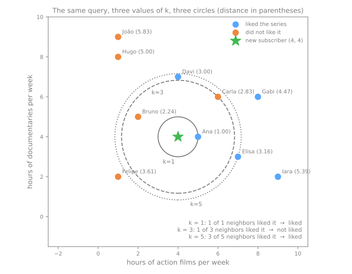
Mesmos dados, mesma consulta, três respostas diferentes. O \(k\) não é um detalhe: é a principal decisão que o k-NN deixa nas suas mãos. O scikit-learn confirma a conta feita à mão:
import numpy as np
import pandas as pd
from sklearn.neighbors import KNeighborsClassifier

users = pd.DataFrame({
    'name':   ['Ana', 'Bruno', 'Carla', 'Davi', 'Elisa', 'Felipe', 'Gabi', 'Hugo', 'Iara', 'João'],
    'action': [5, 2, 6, 4, 7, 1, 8, 1, 9, 1],      # horas de filmes de ação por semana
    'docs':   [4, 5, 6, 7, 3, 2, 6, 8, 2, 9],      # horas de documentários por semana
    'liked':  [1, 0, 0, 1, 1, 0, 1, 0, 1, 0]})     # 1 = gostou da série nova
X, y = users[['action', 'docs']], users['liked']
new = pd.DataFrame({'action': [4], 'docs': [4]})

knn = KNeighborsClassifier(n_neighbors=5).fit(X, y)
dist, idx = knn.kneighbors(new)                    # os 5 mais próximos, em ordem
print(users['name'].iloc[idx[0]].tolist(), dist[0].round(3))

for k in [1, 3, 5]:
    knn = KNeighborsClassifier(n_neighbors=k).fit(X, y)
    print(f"k={k}: predict {knn.predict(new)[0]}   P(liked) = {knn.predict_proba(new)[0, 1]:.3f}")
['Ana', 'Bruno', 'Carla', 'Davi', 'Elisa'] [1.    2.236 2.828 3.    3.162]
k=1: predict 1   P(liked) = 1.000
k=3: predict 0   P(liked) = 0.333
k=5: predict 1   P(liked) = 0.600
O kneighbors devolve os mesmos cinco nomes, na mesma ordem e às mesmas distâncias da tabela. O predict_proba não passa da fração dos \(k\) vizinhos que gostaram da série: 1/1, 1/3 e 3/5.
Ideia-chave
O k-NN não aprende uma fórmula: ele procura os casos mais parecidos com o ponto novo e repete a resposta da maioria deles. Mudar \(k\) muda quem vota e, perto da fronteira, muda a resposta.
2. O algoritmo em três passos
Para classificar um ponto de consulta \(x\):
- calcule a distância de \(x\) a todo ponto de treino;
- fique com os \(k\) mais próximos, a vizinhança \(N_k(x)\);
- preveja a classe mais frequente entre eles. A "probabilidade" da classe \(c\) é a fração dos vizinhos nessa classe:
Na prática, o k-NN sempre entra num pipeline com um escalonador, por motivos que mediremos mais adiante:
from sklearn.neighbors import KNeighborsClassifier
from sklearn.pipeline import make_pipeline
from sklearn.preprocessing import StandardScaler

knn = make_pipeline(StandardScaler(),                 # distâncias precisam de escalonamento!
                    KNeighborsClassifier(n_neighbors=5))
knn.fit(X_train, y_train)
O que o fit guarda: paramétrico vs baseado em instâncias
A regressão logística é um modelo paramétrico: seja qual for o tamanho do conjunto de treino, o que ela aprende cabe em \(d + 1\) números. O k-NN é baseado em instâncias (ou não paramétrico): o que ele "aprende" é o próprio conjunto de treino, então o modelo cresce com os dados.
| regressão logística | k-NN | |
|---|---|---|
o que o fit produz | \(d + 1\) números (\(w\), \(b\)) | uma cópia da tabela de treino \(n \times d\) |
| fronteira de decisão | uma reta (hiperplano) | qualquer forma; segue os dados localmente |
custo do fit | otimização iterativa | quase nenhum: guardar as linhas |
| custo de uma previsão | \(d\) multiplicações | \(n\) distâncias de \(d\) coordenadas cada |
| hiperparâmetros | nenhum na forma pura: você escolhe os atributos | k, a distância, a ponderação |
| sabe dizer por quê | um coeficiente por atributo | "estas \(k\) linhas são as mais parecidas" |
A tabela resume o apelido do k-NN: ele é um aprendiz preguiçoso (lazy). O fit não otimiza nada; no máximo organiza as linhas para acelerar a busca. O trabalho de verdade, calcular a distância da consulta até as linhas guardadas, fica para a hora de prever. A abordagem avançada conta essas distâncias e mostra quanto isso custa.
3. Escalonar não é opcional
Etapa 2. Uma distância soma diferenças nas unidades de cada atributo. Quando as unidades diferem, o atributo com os maiores números decide tudo. Considere seis clientes de uma agência de viagens (uns compraram um pacote de mochilão, outros não) e um cliente novo (R$ 5.000 por mês, 25 anos). Ele vai comprar?
from sklearn.preprocessing import StandardScaler

clients = pd.DataFrame({
    'name':   ['Rita', 'Otávio', 'Sônia', 'Caio', 'Lívia', 'Mário'],
    'income': [5200, 5700, 9000, 3000, 7400, 2600],      # R$ por mês
    'age':    [61, 26, 45, 33, 52, 22],
    'bought': [0, 1, 0, 1, 0, 1]})
F = ['income', 'age']
query = pd.DataFrame({'income': [5000], 'age': [25]})

scaler = StandardScaler().fit(clients[F])
Z, zq = scaler.transform(clients[F]), scaler.transform(query)
clients['d_raw'] = np.sqrt(((clients[F] - query.iloc[0]) ** 2).sum(axis=1)).round(1)
clients['d_scaled'] = np.sqrt(((Z - zq) ** 2).sum(axis=1)).round(2)
print(scaler.scale_.round(1))
print(clients.sort_values('d_raw').to_string(index=False))
[2260.1   14. ]
  name  income  age  bought  d_raw  d_scaled
  Rita    5200   61       0  203.2      2.57
Otávio    5700   26       1  700.0      0.32
  Caio    3000   33       1 2000.0      1.05
 Mário    2600   22       1 2400.0      1.08
 Lívia    7400   52       0 2400.2      2.20
 Sônia    9000   45       0 4000.0      2.27
Confira a Rita à mão: \(\sqrt{200^2 + 36^2} = \sqrt{40.000 + 1.296} = 203{,}2\). A renda dela difere em R$ 200 e a idade em 36 anos; mesmo assim, os 36 anos acrescentam só 3,2 à distância, porque um ano pesa o mesmo que um real. Em unidades brutas, o vizinho mais próximo é uma cliente de 61 anos que não comprou; o 1-NN diz "não".
O StandardScaler divide cada atributo pelo respectivo desvio padrão (R$ 2.260,1 e 14,0 anos aqui; as médias se cancelam numa diferença). Agora a Rita está a \(\sqrt{(200/2260{,}1)^2 + (36/14{,}0)^2} = \sqrt{0{,}09^2 + 2{,}57^2} = 2{,}57\); já o Otávio, de 26 anos, fica a \(\sqrt{(700/2260{,}1)^2 + (1/14{,}0)^2} = 0{,}32\). O vizinho mais próximo passa a ser um cliente de quase a mesma idade que comprou; o 1-NN diz "sim".
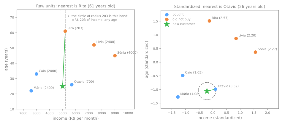
O painel da esquerda conta a história toda: em unidades brutas, um "círculo" de raio 203 em torno do cliente novo é uma faixa de R$ 203 para cada lado que contém todas as idades da figura. Num conjunto de dados real o efeito é igualmente grande. Os 13 atributos do conjunto wine têm dispersões muito diferentes:
from sklearn.datasets import load_wine
from sklearn.model_selection import train_test_split
from sklearn.pipeline import make_pipeline
from sklearn.preprocessing import MinMaxScaler

wine = load_wine(as_frame=True)
print(wine.data.std().sort_values(ascending=False).round(2).head(4))

X_tr, X_te, y_tr, y_te = train_test_split(wine.data, wine.target, test_size=0.3,
                                          stratify=wine.target, random_state=0)
for name, model in [('no scaling', KNeighborsClassifier(5)),
                    ('StandardScaler', make_pipeline(StandardScaler(), KNeighborsClassifier(5))),
                    ('MinMaxScaler', make_pipeline(MinMaxScaler(), KNeighborsClassifier(5)))]:
    print(f"{name:15s} {model.fit(X_tr, y_tr).score(X_te, y_te):.3f}")
proline              314.91
magnesium             14.28
alcalinity_of_ash      3.34
color_intensity        2.32
dtype: float64
no scaling      0.722
StandardScaler  0.963
MinMaxScaler    0.963
A proline tem desvio padrão de 315, mais de vinte vezes o de qualquer outro atributo, então a distância bruta é basicamente a diferença de prolina: o 5-NN está classificando vinhos por uma única coluna entre 13. Ele acerta 72,2% dos 54 vinhos de teste (39). Coloque os atributos numa escala comum e o mesmo 5-NN acerta 96,3% (52). Padronização e min-max se saem igualmente bem aqui; o que importa é que nenhum atributo domine por um acidente de unidade.
Escalone primeiro, sempre dentro de um pipeline
k-NN sem escalonamento é um bug, não um modelo (a menos que todos os atributos já compartilhem uma unidade, como os pixels do lab avançado). O escalonador precisa aprender médias e desvios padrão só das linhas de treino e depois ser aplicado, sem reajuste, à validação e ao teste. make_pipeline(StandardScaler(), KNeighborsClassifier()) faz exatamente isso (Pipelines).
4. Escolher \(k\): viés e variância
Etapa 3. O \(k\) controla a complexidade. Um \(k\) pequeno consulta pouquíssimos pontos, então a fronteira se curva em torno de cada um; um \(k\) grande faz a média sobre uma região grande, então a fronteira fica suave. É o trade-off viés–variância com o sentido invertido: \(k\) pequeno = modelo complexo. Para ver isso, tome um conjunto de duas luas com ruído (1.000 pontos) e divida em 600 de treino, 200 de validação e 200 de teste:
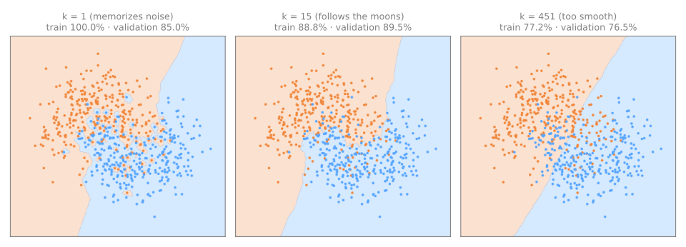
- \(k = 1\): cada ponto de treino governa sua própria ilha. A fronteira memoriza o ruído; a acurácia de treino é 100% e a de validação 85,0%: variância alta, sobreajuste;
- \(k = 15\): uma fronteira suave que segue as duas luas, 89,5% na validação;
- \(k = 451\) (três quartos do conjunto de treino): cada votação é dominada por pontos distantes e a fronteira é quase uma reta: viés alto, subajuste. Com \(k = n\), toda consulta recebe os mesmos vizinhos e o k-NN prevê a classe majoritária em todo lugar.
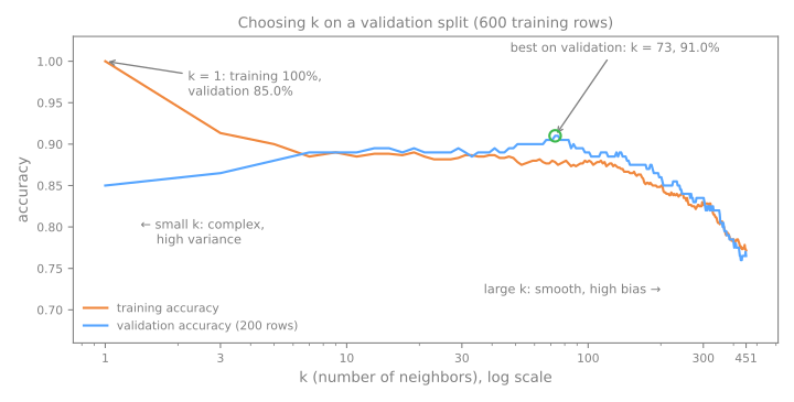
Para escolher \(k\), avalie cada candidato na divisão de validação. O teste fica intocado até o final:
from sklearn.datasets import make_moons

X, y = make_moons(n_samples=1000, noise=0.35, random_state=0)
X_tmp, X_test, y_tmp, y_test = train_test_split(X, y, test_size=0.2, stratify=y, random_state=0)
X_train, X_val, y_train, y_val = train_test_split(X_tmp, y_tmp, test_size=0.25,
                                                  stratify=y_tmp, random_state=0)
print(len(X_train), len(X_val), len(X_test))

rows = []
for k in range(1, 452, 2):                                   # todo k ímpar até 451
    m = KNeighborsClassifier(n_neighbors=k).fit(X_train, y_train)
    rows.append((k, m.score(X_train, y_train), m.score(X_val, y_val)))
table = pd.DataFrame(rows, columns=['k', 'train', 'validation'])
print(table[table['k'].isin([1, 3, 5, 9, 15, 31, 51, 73, 101, 151, 301, 451])]
      .round(3).to_string(index=False))
600 200 200
  k  train  validation
  1  1.000       0.850
  3  0.913       0.865
  5  0.900       0.880
  9  0.890       0.890
 15  0.888       0.895
 31  0.887       0.890
 51  0.878       0.900
 73  0.878       0.910
101  0.880       0.890
151  0.865       0.875
301  0.827       0.835
451  0.772       0.765
Como ler:
- A acurácia de treino em \(k = 1\) é 100% por construção. Cada ponto de treino é o seu próprio vizinho mais próximo, a distância 0, então ele sempre vota no próprio rótulo. Esse número não diz nada sobre dados novos. O escore de validação, 85,0%, diz.
- O platô. De \(k = 7\) até \(k \approx 140\), a acurácia de validação fica entre 88,5% e 91,0%. Com 200 linhas de validação, uma linha vale 0,5 ponto, então o platô inteiro cabe em 5 linhas: os dados mal distinguem esses valores de \(k\). A regra de bolso \(k \approx \sqrt{n} = \sqrt{600} \approx 24\) também cai no platô, mas meça em vez de confiar nela.
- \(k\) grande. A partir de \(k \approx 150\), treino e validação caem juntos. Quando os dois estão baixos e próximos, o modelo é simples demais.
Escolha o melhor escore de validação, reajuste em treino + validação e meça o teste uma vez:
best_k = int(table.loc[table['validation'].idxmax(), 'k'])
final = KNeighborsClassifier(n_neighbors=best_k).fit(X_tmp, y_tmp)   # treino + validação
print(f"chosen k = {best_k} · test accuracy {final.score(X_test, y_test):.3f}")
O escore de teste (90,0%) fica um ponto abaixo do escore de validação vencedor (91,0%). Isso é esperado: \(k = 73\) foi escolhido porque se saiu melhor naquelas 200 linhas, então parte dos seus 91,0% é sorte. O teste, usado uma vez, dá a estimativa honesta. Escolher \(k\) no teste destruiria justamente essa honestidade. Uma única divisão de validação também é ruidosa por si só: a validação cruzada, daqui a algumas aulas, vai tornar essa escolha mais robusta.
Use \(k\) ímpar com duas classes. Com \(k\) par, a votação pode empatar (1 a 1, 2 a 2) e a regra de desempate do scikit-learn não é a que você imaginaria; a abordagem avançada mostra qual é.
O ponto de consulta ★ começa bem na fronteira entre as classes. Sem movê-lo, percorra o \(k\) de 1 a 25: com \(k = 1\) e \(k = 3\) ele é azul, de 5 a 15 vira laranja e, a partir de 17, volta a ser azul. Perto da fronteira, a resposta depende de quantos vizinhos votam. Depois arraste o ponto pela zona em que as classes se sobrepõem: o \(k\) pequeno oscila a cada movimento, enquanto o \(k\) grande permanece estável.
5. Resumo: a receita do k-NN
- Monte um pipeline com o escalonador e o k-NN:
make_pipeline(StandardScaler(), KNeighborsClassifier()). - Divida antes de olhar resultados: treino (as linhas que votam), validação (para escolher \(k\)) e teste (trancado até o fim).
- Varra \(k\) ímpar na validação. Desconfie dos 100% de treino com \(k = 1\): são garantidos por construção.
- Reajuste em treino + validação com o \(k\) escolhido e meça o teste uma única vez.
| erro comum | sintoma | correção |
|---|---|---|
| k-NN sem escalonador | a resposta muda quando uma coluna muda de unidade | escalonador dentro do pipeline |
| escalonador ajustado em todas as linhas | a validação já viu médias e desvios das linhas que deveria julgar (vazamento) | ajustar o escalonador só no treino: o pipeline faz isso |
| escolher \(k\) pela acurácia de treino | \(k = 1\) sempre "vence", com 100% | escolher na validação |
| escolher \(k\) no teste | o número final deixa de ser uma estimativa honesta | tocar o teste uma única vez, no final |
Lab fundamental — vinhos
O conjunto wine vem com o scikit-learn: 178 vinhos, 13 medidas químicas, 3 cultivares. Nos passos 1 a 5 você abre o k-NN por dentro: vê as unidades decidirem a distância, olha os vizinhos de um vinho votarem, reescreve o método em quatro linhas de NumPy e escolhe \(k\) numa divisão de validação.
Como fazer este lab em aula (cerca de 35 min, em duplas)
- Abra o notebook do lab no Colab. Não é preciso baixar nem instalar nada: o Colab roda no navegador. Para guardar as suas respostas, salve uma cópia no seu Drive (Arquivo → Salvar uma cópia no Drive) antes de editar. Rode as células em ordem, numa mesma sessão.
- Este lab corresponde aos passos 1 a 5 do notebook. O lab avançado continua no mesmo notebook, a partir do passo 6.
- Cada passo começa com um Preveja: responda com a dupla antes de rodar a célula. Errar a previsão é o que torna o resultado memorável.
- Depois de rodar, compare com a saída e a leitura desta página. Toda saída aqui é exatamente o que o código imprime.
- As Simulações pedem que vocês escrevam um pequeno experimento em Python: mudar uma entrada do modelo e observar o que acontece com a saída. Nada de conta à mão. A solução fica recolhida logo abaixo: tente antes de abrir.
- Ritmo sugerido: passos 1 a 3 em 15 min; passos 4 e 5 em 20 min.
Passo 1 — carregar os vinhos e olhar as unidades
Preveja. Numa distância euclidiana entre dois vinhos, qual destes quatro atributos vai pesar mais: teor alcoólico, tonalidade (hue), magnésio ou prolina? Por quê?
import numpy as np
import pandas as pd
import matplotlib.pyplot as plt
from sklearn.datasets import load_wine

wine = load_wine(as_frame=True)
X, y = wine.data, wine.target        # 13 medidas químicas; 3 cultivares (0, 1, 2)
print(X.shape)
print(y.value_counts().sort_index().to_dict())
print(X[['alcohol', 'hue', 'magnesium', 'proline']].agg(['min', 'max', 'std']).round(2))
(178, 13)
{0: 59, 1: 71, 2: 48}
     alcohol   hue  magnesium  proline
min    11.03  0.48      70.00   278.00
max    14.83  1.71     162.00  1680.00
std     0.81  0.23      14.28   314.91
178 vinhos de três cultivares, mais ou menos equilibrados (71 no mais frequente). Olhe as unidades antes de modelar: hue varia 0,23 (um desvio padrão), proline varia 315. Uma distância soma as diferenças nas unidades de cada coluna, então, sem escalonamento, uma diferença de uma unidade de prolina (0,3% do seu desvio padrão) conta o mesmo que uma diferença de uma unidade de tonalidade (mais de quatro desvios padrão dela). A prolina vai mandar.
Passo 2 — dividir em treino, validação e teste
Preveja. Para que serve cada uma das três partes? Qual delas o k-NN vai guardar dentro de si no fit?
from sklearn.model_selection import train_test_split

X_tmp, X_test, y_tmp, y_test = train_test_split(X, y, test_size=0.2, stratify=y, random_state=42)
X_train, X_val, y_train, y_val = train_test_split(X_tmp, y_tmp, test_size=0.25,
                                                  stratify=y_tmp, random_state=42)
print(len(X_train), len(X_val), len(X_test))
Uma divisão 60/20/20: 106 vinhos de treino (são eles que o k-NN guarda e que vão votar), 36 de validação (para escolher \(k\)) e 36 de teste, trancados para a medida final. O stratify mantém as proporções de cultivares iguais nas três partes. Com 36 vinhos de validação, um vinho vale 2,8 pontos de acurácia; lembre-se disso ao ler as diferenças.
Passo 3 — baseline e o preço de pular o escalonador
Preveja. O mesmo 5-NN, com e sem o StandardScaler: qual acerta mais na validação? A diferença vai ser de um ou dois vinhos ou bem maior?
from sklearn.dummy import DummyClassifier
from sklearn.neighbors import KNeighborsClassifier
from sklearn.pipeline import make_pipeline
from sklearn.preprocessing import StandardScaler

models = {
    'baseline (majoritária)': DummyClassifier(strategy='most_frequent'),
    'k-NN, atributos brutos': KNeighborsClassifier(n_neighbors=5),
    'k-NN, padronizado':      make_pipeline(StandardScaler(), KNeighborsClassifier(n_neighbors=5)),
}
for name, model in models.items():
    model.fit(X_train, y_train)
    print(f"{name:23s} acurácia de validação {model.score(X_val, y_val):.3f}")
baseline (majoritária)  acurácia de validação 0.389
k-NN, atributos brutos  acurácia de validação 0.694
k-NN, padronizado       acurácia de validação 0.972
Como ler:
- Baseline. Responder sempre o cultivar mais frequente acerta 38,9% (14 de 36). Qualquer modelo precisa superar isso.
- Atributos brutos. O 5-NN nas medidas brutas acerta 69,4%: melhor que a baseline, mas ele está medindo basicamente a prolina.
- Padronizado. O mesmo 5-NN depois do
StandardScaleracerta 97,2%, 35 de 36. O escalonador está dentro do pipeline, então suas médias e desvios padrão vêm só dos 106 vinhos de treino.
Simulação: a unidade da prolina. A prolina está em mg/L. Reescreva-a em g/L (divida a coluna por 1.000, no treino e na validação) e rode de novo o 5-NN bruto e o padronizado. São os mesmos vinhos, com a mesma informação. O que muda em cada modelo? Qual coluna passa a mandar na distância bruta?
Solução
for unit, factor in [('mg/L', 1), ('g/L', 1 / 1000)]:
    Xa, Xb = X_train.copy(), X_val.copy()
    Xa['proline'] *= factor                          # mesma medida, outra unidade
    Xb['proline'] *= factor
    raw = KNeighborsClassifier(n_neighbors=5).fit(Xa, y_train).score(Xb, y_val)
    std = make_pipeline(StandardScaler(), KNeighborsClassifier(n_neighbors=5)).fit(Xa, y_train).score(Xb, y_val)
    print(f"prolina em {unit:4s}: bruto {raw:.3f} · padronizado {std:.3f} · "
          f"maior desvio padrão: {Xa.std().idxmax()}")
prolina em mg/L: bruto 0.694 · padronizado 0.972 · maior desvio padrão: proline
prolina em g/L : bruto 0.861 · padronizado 0.972 · maior desvio padrão: magnesium
Só trocar a unidade de uma coluna leva o k-NN bruto de 69,4% para 86,1%: nenhum vinho mudou, só a régua. Com a prolina em g/L, quem passa a mandar na distância é o magnésio, o próximo da fila em desvio padrão. Um modelo cuja resposta depende da unidade em que alguém anotou a planilha não está medindo semelhança. O k-NN padronizado não se mexe (97,2% nos dois casos): o StandardScaler divide cada coluna pelo seu desvio padrão e isso apaga a unidade.
Passo 4 — o k-NN por dentro: os vizinhos votam
Preveja. O fit da regressão logística aprendia um peso por atributo. O que o fit do k-NN guarda? Se os 5 vizinhos de um vinho são dos cultivares 0, 1, 0, 1, 0, o que o predict_proba devolve?
knn5 = make_pipeline(StandardScaler(), KNeighborsClassifier(n_neighbors=5)).fit(X_train, y_train)
print(f"o fit guardou {knn5[-1].n_samples_fit_} linhas de {knn5[-1].n_features_in_} atributos")

wine_id = 123                                        # um vinho da validação
query = X_val.loc[[wine_id]]
dist, idx = knn5[-1].kneighbors(knn5[0].transform(query))
print(pd.DataFrame({'vizinho': X_train.index[idx[0]], 'distância': dist[0].round(2),
                    'cultivar': y_train.iloc[idx[0]].to_numpy()}).to_string(index=False))
print("votos por cultivar:", np.bincount(y_train.iloc[idx[0]], minlength=3))
print("predict_proba:", knn5.predict_proba(query)[0], "· predict:", knn5.predict(query)[0],
      "· verdade:", y_val[wine_id])
o fit guardou 106 linhas de 13 atributos
 vizinho  distância  cultivar
      43       2.86         0
     124       3.03         1
      41       3.32         0
     122       3.73         1
      21       3.78         0
votos por cultivar: [3 2 0]
predict_proba: [0.6 0.4 0. ] · predict: 0 · verdade: 1
O fit não aprendeu peso nenhum: guardou os 106 vinhos de treino, padronizados. Para prever, o k-NN mede a distância do vinho 123 a cada um deles e fica com os 5 mais próximos. Três são do cultivar 0 e dois do cultivar 1, então o predict_proba é só a contagem de votos dividida por 5 (0,6 e 0,4) e o predict é o cultivar mais votado, 0. Aqui ele erra: o vinho 123 é do cultivar 1. Repare nas distâncias: os cinco vizinhos estão entre 2,86 e 3,78, nenhum muito mais perto que os outros. O vinho está numa zona em que os dois cultivares se misturam.
O método inteiro cabe em quatro linhas de NumPy: distâncias, ordenar, pegar os \(k\) primeiros, votar.
Z_train, Z_val = knn5[0].transform(X_train), knn5[0].transform(X_val)
D = np.sqrt(((Z_val[:, None, :] - Z_train[None, :, :]) ** 2).sum(axis=2))   # distância de cada vinho
nearest = np.argsort(D, axis=1)[:, :5]                                      # de validação a cada vinho
votes = y_train.to_numpy()[nearest]                                         # de treino
mine = np.array([np.bincount(v, minlength=3).argmax() for v in votes])
print(D.shape, "· igual ao scikit-learn:", (mine == knn5.predict(X_val)).all())
Uma matriz de 36 × 106 distâncias, uma por par (vinho de validação, vinho de treino): todo o trabalho acontece na hora de prever. As previsões são idênticas às do scikit-learn. O que a biblioteca acrescenta é velocidade (árvores de busca, código compilado) e conveniências, não outro algoritmo.
Simulação: o voto muda com \(k\). Para o vinho 123, peça os 15 vizinhos mais próximos de uma vez e, para \(k\) = 1, 3, 5, 7, 9, 11, 13 e 15, conte os votos dos \(k\) primeiros e imprima a previsão. Com que \(k\) a previsão fica certa?
Solução
dist, idx = knn5[-1].kneighbors(knn5[0].transform(query), n_neighbors=15)
labels = y_train.iloc[idx[0]].to_numpy()                # cultivares, do mais perto ao mais longe
print("cultivares dos 15 vizinhos:", labels)
for k in range(1, 16, 2):
    votes = np.bincount(labels[:k], minlength=3)
    print(f"k={k:2d}: votos {votes} -> previsão {votes.argmax()}")
cultivares dos 15 vizinhos: [0 1 0 1 0 1 1 1 1 1 1 1 0 1 1]
k= 1: votos [1 0 0] -> previsão 0
k= 3: votos [2 1 0] -> previsão 0
k= 5: votos [3 2 0] -> previsão 0
k= 7: votos [3 4 0] -> previsão 1
k= 9: votos [3 6 0] -> previsão 1
k=11: votos [3 8 0] -> previsão 1
k=13: votos [4 9 0] -> previsão 1
k=15: votos [ 4 11  0] -> previsão 1
Com \(k\) = 1, 3 e 5 o vinho é classificado como cultivar 0; a partir de \(k = 7\), como cultivar 1, o certo. Os vizinhos mais próximos são uma amostra pequena e ruidosa da vizinhança; somar mais votos faz a média sobre uma região maior. É o mesmo movimento do simulador acima: perto da fronteira, a resposta depende de quantos vizinhos votam. O passo 5 escolhe \(k\) olhando todos os 36 vinhos de validação de uma vez, não um só.
Passo 5 — escolher \(k\) na validação e testar uma vez
Preveja. Com \(k = 1\), quanto dá a acurácia de treino? Esse número diz algo sobre vinhos novos?
rows = []
for k in range(1, 32, 2):
    model = make_pipeline(StandardScaler(), KNeighborsClassifier(n_neighbors=k))
    model.fit(X_train, y_train)
    val_acc = model.score(X_val, y_val)
    rows.append({'k': k, 'treino': model.score(X_train, y_train), 'validação': val_acc,
                 'erros val': round((1 - val_acc) * len(y_val))})
table = pd.DataFrame(rows)
print(table.round(3).to_string(index=False))
best_k = int(table.loc[table['validação'].idxmax(), 'k'])   # primeiro (menor) k com o melhor escore

final = make_pipeline(StandardScaler(), KNeighborsClassifier(n_neighbors=best_k))
final.fit(X_tmp, y_tmp)                                      # treino + validação, mesma receita
print(f"k escolhido: {best_k} · acurácia de teste {final.score(X_test, y_test):.3f} em {len(y_test)} vinhos")
 k  treino  validação  erros val
 1   1.000      0.944          2
 3   0.972      0.972          1
 5   0.972      0.972          1
 7   0.953      1.000          0
 9   0.962      1.000          0
11   0.962      1.000          0
13   0.972      1.000          0
15   0.962      1.000          0
17   0.962      1.000          0
19   0.972      1.000          0
21   0.972      1.000          0
23   0.972      1.000          0
25   0.972      1.000          0
27   0.972      1.000          0
29   0.962      1.000          0
31   0.962      1.000          0
k escolhido: 7 · acurácia de teste 1.000 em 36 vinhos
Como ler:
- \(k = 1\) tem 100% de acurácia de treino por construção: cada vinho de treino é o seu próprio vizinho mais próximo, a distância 0, e vota no próprio rótulo. Na validação ele faz o pior escore, 2 erros. É a marca do sobreajuste.
- De \(k = 7\) a 31, a validação é perfeita. Os dados não conseguem distinguir esses valores: a diferença entre \(k = 5\) e \(k = 7\) é um único vinho (o 123 do passo 4). O
idxmaxdevolve o primeiro máximo, então ficamos com o menor \(k\) do platô, 7; qualquer valor do platô seria uma escolha defensável. - O teste. A receita escolhida (padronizar, depois 7-NN) é reajustada nos 142 vinhos de treino + validação e só agora encontra o teste: 36 acertos em 36. Resista à tentação de voltar e "melhorar" o \(k\) depois de ver esse número: a partir daí o teste seria um segundo conjunto de validação.
Para fechar a parte fundamental. Em uma frase cada: (1) o que o fit do k-NN guarda e em que momento acontece o trabalho de verdade? (2) Por que o k-NN sem escalonamento mudou de resposta quando a prolina mudou de unidade? (3) Por que a acurácia de treino com \(k = 1\) não serve para escolher \(k\)?
Sua vez (fundamental)
Para casa:
- Outros escalonadores. Refaça o passo 3 trocando o
StandardScalerporMinMaxScalere porRobustScaler. A acurácia de validação muda? Por que os três resolvem o problema da prolina? - Escolher pelo treino. No passo 5, escolha \(k\) pela coluna
treinoem vez da colunavalidação. Que \(k\) sai? Por que essa escolha é ruim? - Outra divisão. Troque
random_state=42por outros valores no passo 2 e refaça os passos 3 e 5. O \(k\) escolhido muda? O que isso diz sobre confiar numa única divisão de validação? (A validação cruzada resolve isso mais adiante.)
Abordagem avançada
A abordagem fundamental terminou com uma receita que funciona: escalonar, escolher \(k\) na validação, testar uma vez. Esta parte pergunta onde a receita quebra, quanto ela custa e quando outro modelo é melhor. Os blocos de código continuam os das seções 1 a 5 (o código dos labs roda à parte, no Colab): os assinantes (users, new), as luas (X, y, X_train, X_val, y_train, y_val) e os vinhos (wine) já estão definidos.
Esta parte segue quatro etapas, desenhadas abaixo: 1. escolher a distância; 2. como o voto conta (empates, pesos, predict_proba); 3. onde o k-NN quebra (dimensão alta e custo de prever); 4. quando usar, contra a regressão logística e na regressão. Cada etapa leva à sua seção e, nos slides, uma faixa embaixo mostra em que etapa você está.
- Escolher a distânciaMinkowski, cosseno, Hamming: pelo tipo de dado
- Como o voto contaempates, pesos 1/d, um
predict_probagrosseiro - Onde quebraa maldição da dimensionalidade; o custo de prever
- Quando usarcontra a regressão logística; regressão; perfil prático
Slides da abordagem avançada
Clique nos slides e use as setas ← → para navegar; F abre em tela cheia e Esc mostra todos os slides. Abrir os slides numa aba nova
6. Distância: o que "perto" significa
Etapa 1. "Parecido" precisa virar um número; essa escolha faz parte do modelo. A família padrão é a distância de Minkowski de ordem \(p\):
Tome \(a = (1, 2)\) e \(b = (4, 6)\). As diferenças por coordenada são 3 e 4.
- \(p = 1\), Manhattan: some as diferenças, \(3 + 4 = 7\). A distância que um táxi percorre numa malha de ruas;
- \(p = 2\), euclidiana: \(\sqrt{3^2 + 4^2} = 5\). A linha reta, padrão do scikit-learn;
- \(p = \infty\), Chebyshev: só a maior diferença conta, \(\max(3, 4) = 4\).
from sklearn.metrics import pairwise_distances

a, b = np.array([[1, 2]]), np.array([[4, 6]])
for metric in ['manhattan', 'euclidean', 'chebyshev']:
    print(f"{metric:10s} {pairwise_distances(a, b, metric=metric)[0, 0]:.1f}")
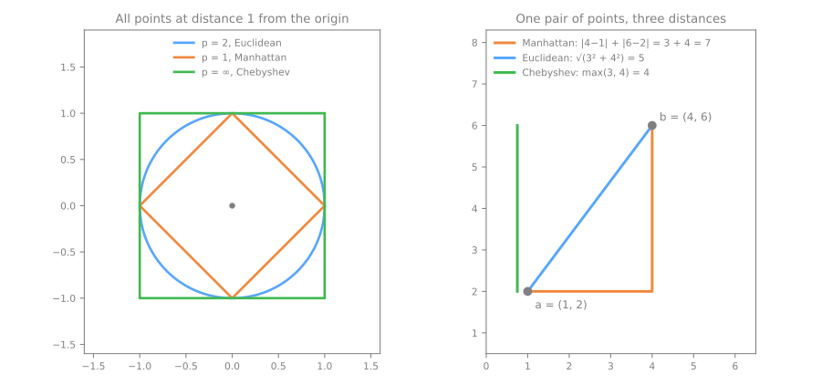
O painel da esquerda mostra o que cada distância chama de "vizinhança": o conjunto dos pontos a distância 1 é um losango, um círculo ou um quadrado. Elevar ao quadrado deixa a distância euclidiana sensível a uma diferença grande num único atributo. Manhattan soma as diferenças sem elevá-las ao quadrado, então nenhum atributo domina com tanta facilidade. Chebyshev só olha o pior atributo. No scikit-learn: KNeighborsClassifier(p=1) ou metric='manhattan', p=2 (o padrão), metric='chebyshev'.
Outras duas distâncias que você vai encontrar:
- A distância de cosseno (\(1 - \cos\theta\)) compara a direção de dois vetores e ignora o comprimento. Os vetores \((1, 1, 0)\) e \((10, 10, 0)\) estão a 12,7 de distância euclidiana, mas a distância de cosseno 0: o mesmo "assunto", só que um é mais longo. É o que se quer para contagens de palavras e embeddings (Representação de Texto), em que um documento longo não deve ficar longe de um curto sobre o mesmo tema. Use
metric='cosine'. - A distância de Hamming conta as posições em que dois vetores binários diferem. Categorias nominais precisam de one-hot antes: codificar
vermelho, verde, azulcomo 0, 1, 2 deixaria vermelho "mais perto" de verde do que de azul, uma distância fictícia.
Em resumo, a escolha depende do tipo de dado:
| tipo de dado | distância | por quê |
|---|---|---|
| atributos numéricos, já escalonados | euclidiana (o padrão) | a linha reta; funciona bem quando todos os atributos importam |
| atributos numéricos com diferenças grandes e isoladas | Manhattan | soma sem elevar ao quadrado: um atributo sozinho domina menos |
| contagens de palavras, TF-IDF, embeddings | cosseno | compara a direção e ignora o comprimento |
| vetores binários (one-hot, presença/ausência) | Hamming | conta as posições em que os vetores diferem |
Na dúvida, trate a distância como um hiperparâmetro e compare as opções na validação, como se faz com \(k\).
7. Empates, votos ponderados e o predict_proba
Etapa 2. Com duas classes, um \(k\) ímpar nunca produz empate na votação. Com \(k\) par, pode produzir. O scikit-learn não desempata pela distância: ele devolve a classe que vem primeiro em classes_. No exemplo dos assinantes com \(k = 2\), Ana (sim) e Bruno (não) empatam e a previsão é "não gostou" (classe 0), embora a vizinha mais próxima tenha gostado da série (veja o próximo bloco). Com três ou mais classes, um \(k\) ímpar já não garante nada (5 votos podem se dividir em 2–2–1). Empates de distância (dois pontos de treino exatamente à mesma distância da consulta disputando a última vaga) são resolvidos pela ordem das linhas nos dados de treino.
Com weights='distance', cada vizinho vota com peso \(1/d\), então os mais próximos contam mais. Refaça \(k = 3\) para o assinante novo à mão: Ana pesa \(1/1 = 1{,}000\), Bruno \(1/2{,}236 = 0{,}447\), Carla \(1/2{,}828 = 0{,}354\). "Gostou" recebe 1,000 e "não gostou" recebe \(0{,}447 + 0{,}354 = 0{,}801\); portanto
X_u, y_u = users[['action', 'docs']], users['liked']
for k in [2, 3]:
    for w in ['uniform', 'distance']:
        m = KNeighborsClassifier(n_neighbors=k, weights=w).fit(X_u, y_u)
        print(f"k={k} {w:8s} predict {m.predict(new)[0]}   P(liked) = {m.predict_proba(new)[0, 1]:.3f}")
k=2 uniform  predict 0   P(liked) = 0.500
k=2 distance predict 1   P(liked) = 0.691
k=3 uniform  predict 0   P(liked) = 0.333
k=3 distance predict 1   P(liked) = 0.555
A ponderação inverte as duas respostas: a Ana está bem mais perto que Bruno e Carla; agora isso conta. Ela também desfaz o empate de \(k = 2\) (\(1/(1 + 0{,}447) = 0{,}691\)). A ponderação por distância deixa o k-NN menos sensível à escolha exata de \(k\), porque vizinhos distantes contam pouco; trate weights como um segundo hiperparâmetro e escolha-o também na validação.
Com pesos uniformes, o predict_proba é uma fração de \(k\) vizinhos, então só pode assumir os \(k + 1\) valores \(0, 1/k, 2/k, \ldots, 1\):
for k in [5, 15, 73]:
    proba = KNeighborsClassifier(n_neighbors=k).fit(X_train, y_train).predict_proba(X_val)[:, 1]
    print(f"k={k:2d}: {len(np.unique(proba)):2d} distinct probabilities, e.g. {np.unique(proba)[:4].round(3)}")
k= 5:  6 distinct probabilities, e.g. [0.  0.2 0.4 0.6]
k=15: 16 distinct probabilities, e.g. [0.    0.067 0.133 0.2  ]
k=73: 62 distinct probabilities, e.g. [0.    0.014 0.027 0.041]
Com \(k = 5\), os 200 pontos de validação compartilham apenas 6 probabilidades possíveis. São escores grosseiros, não a saída suave de uma sigmoide. Guarde isso para as próximas aulas, em que as métricas e as curvas ROC deslocam um limiar de decisão sobre os escores: com o 5-NN há só 6 lugares para colocá-lo.
8. A maldição da dimensionalidade
Etapa 3. O k-NN se apoia numa premissa: perto significa parecido. Em muitas dimensões essa premissa falha, de duas maneiras mensuráveis. (A aula de redução de dimensionalidade tem um simulador da primeira.)
As distâncias se concentram. Espalhe 1.000 pontos aleatórios no cubo unitário, sorteie 100 pontos de consulta e compare o vizinho mais próximo e o mais distante de cada consulta (a mediana sobre as 100 consultas descreve uma consulta típica):
for d in [2, 10, 100, 1000]:
    rng = np.random.default_rng(d)
    P = rng.uniform(size=(1000, d))                     # 1000 pontos aleatórios no cubo unitário
    Q = rng.uniform(size=(100, d))                      # 100 pontos de consulta
    D = pairwise_distances(Q, P)                        # 100 x 1000 distâncias
    near, far = D.min(axis=1), D.max(axis=1)            # para cada consulta
    print(f"d={d:4d}  nearest {np.median(near):6.3f}  farthest {np.median(far):6.3f}  "
          f"(far - near)/near = {np.median((far - near) / near):6.2f}")   # consulta típica
d=   2  nearest  0.014  farthest  1.044  (far - near)/near =  71.21
d=  10  nearest  0.505  farthest  1.894  (far - near)/near =   2.69
d= 100  nearest  3.311  farthest  4.755  (far - near)/near =   0.44
d=1000  nearest 12.188  farthest 13.611  (far - near)/near =   0.12
Em 2 dimensões, uma consulta típica tem o ponto mais próximo a 0,014 e o mais distante a 1,044: a diferença entre eles é 71 vezes a distância do mais próximo, então "mais próximo" destaca algo que faz sentido. Em 1.000 dimensões o ponto mais próximo está a 12,2 e o mais distante a 13,6, uma diferença de só 12%. Todos os pontos estão mais ou menos igualmente longe; os \(k\) "mais próximos" mal estão mais perto que o resto. Beyer et al. (1999) provaram que, à medida que \(d\) cresce, isso acontece para uma classe ampla de distribuições de dados, não só para ruído uniforme. O painel da esquerda da figura abaixo traça a mesma razão para mais valores de \(d\).
Atributos irrelevantes afogam os úteis. Dados reais não têm 1.000 dimensões de sinal, mas muitas vezes têm várias colunas que não carregam sinal nenhum. Acrescente colunas de puro ruído aos 13 atributos do wine e compare o k-NN com a regressão logística:
from sklearn.linear_model import LogisticRegression

rng = np.random.default_rng(0)
Xw, yw = wine.data.to_numpy(), wine.target.to_numpy()
print("noise cols   k-NN   logistic")
for n_noise in [0, 10, 100, 1000]:
    Xn = np.hstack([Xw, rng.normal(size=(len(Xw), n_noise))])   # acrescenta colunas de puro ruído
    a, b, c, d = train_test_split(Xn, yw, test_size=0.3, stratify=yw, random_state=0)
    knn_acc = make_pipeline(StandardScaler(), KNeighborsClassifier(5)).fit(a, c).score(b, d)
    log_acc = make_pipeline(StandardScaler(), LogisticRegression(max_iter=2000)).fit(a, c).score(b, d)
    print(f"{n_noise:10d}   {knn_acc:.3f}  {log_acc:.3f}")
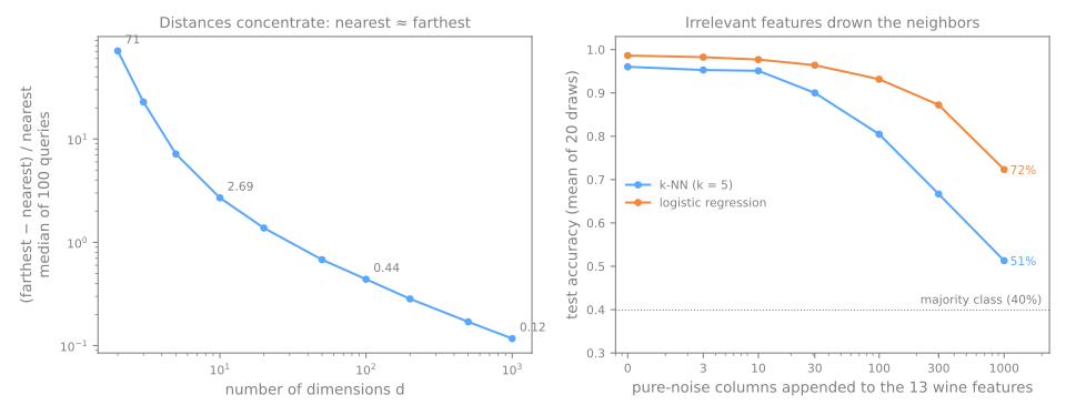
Uma única divisão é ruidosa (a regressão logística perde 5,6 pontos com 10 colunas de ruído por puro acaso), então o painel da direita faz a média de 20 sorteios de ruído e de divisão. O padrão é claro: com 100 colunas de ruído o k-NN cai para 80% em média, com 1.000 para 51%, pouco acima dos 40% de responder sempre o cultivar majoritário. O motivo está na fórmula. Uma distância euclidiana soma uma diferença ao quadrado por coluna — e toda coluna conta igual. Depois da padronização, 1.000 colunas de ruído contribuem cerca de 77 vezes mais para a distância do que as 13 reais, então os vizinhos são escolhidos pelo ruído. A regressão logística aprende um peso por coluna e pode empurrar os pesos do ruído para perto de zero, ajudada aqui pela penalidade L2 padrão do scikit-learn (a que a aula de regressão logística desligou com C=np.inf), que mantém os pesos pequenos; ela também se degrada, mas bem mais tarde.
Remédios: manter só os atributos relevantes (seleção de atributos, conhecimento do domínio), comprimir com PCA antes do k-NN ou aprender a própria distância (metric learning). O k-NN brilha com muitos dados e poucas dimensões, todas com significado.
9. Custo na hora da previsão
Como a seção 2 adiantou, o k-NN é um aprendiz preguiçoso (lazy): o fit adia todo o trabalho para a hora da previsão. Cronometrar daria números que dependem da máquina; por isso, vamos contar as distâncias calculadas. A distância abaixo é a euclidiana de sempre, com um contador acrescentado:
import numpy as np

calls = 0
def euclidean(a, b):                     # a distância de sempre, mais um contador
    global calls
    calls += 1
    return np.sqrt(((a - b) ** 2).sum())

rng_demo = np.random.default_rng(0)
X_big = rng_demo.uniform(size=(2000, 2)); y_big = (X_big[:, 0] > 0.5).astype(int)
queries = rng_demo.uniform(size=(20, 2))

knn = KNeighborsClassifier(n_neighbors=5, algorithm='brute', metric=euclidean)
knn.fit(X_big, y_big);   print(f"fit:     {calls:6d} distances")
calls = 0
knn.predict(queries);    print(f"predict: {calls:6d} distances for {len(queries)} queries")
O ajuste em 2.000 linhas não calculou nada. Cada uma das 20 previsões calculou 2.000 distâncias, uma por linha guardada. O custo de uma previsão é \(O(n \cdot d)\): dobre o conjunto de treino e cada previsão custa o dobro. É o perfil oposto ao da regressão logística, que faz todo o trabalho no fit e depois prevê quase de graça.
A força bruta compara a consulta com cada linha guardada. Árvores de busca (algorithm='kd_tree' ou 'ball_tree') organizam os pontos de treino em regiões aninhadas na hora do fit, de modo que uma consulta pode pular regiões inteiras que comprovadamente estão longe demais. Com a distância com contador de antes:
for d in [2, 10, 50]:
    Xd = rng.uniform(size=(2000, d)); yd = (Xd[:, 0] > 0.5).astype(int)
    Qd = rng.uniform(size=(20, d))
    for algo in ['brute', 'ball_tree']:
        knn = KNeighborsClassifier(n_neighbors=5, algorithm=algo, metric=euclidean).fit(Xd, yd)
        calls = 0
        knn.predict(Qd)
        print(f"d={d:2d} {algo:9s} {calls / len(Qd):6.0f} distances per query")
d= 2 brute       2000 distances per query
d= 2 ball_tree    118 distances per query
d=10 brute       2000 distances per query
d=10 ball_tree   2124 distances per query
d=50 brute       2000 distances per query
d=50 ball_tree   2127 distances per query
Em 2 dimensões, a ball tree acha os 5 mais próximos entre 2.000 pontos com 118 cálculos de distância em vez de 2.000, 17 vezes menos. Em 10 e 50 dimensões ela calcula mais do que a força bruta: quando todas as distâncias são parecidas (a concentração vista acima), nenhuma região pode ser descartada e a árvore ainda acrescenta o próprio custo. O padrão algorithm='auto' escolhe um método a partir do formato dos dados.
Para milhões de linhas em centenas de dimensões (embeddings de imagem ou de texto), a busca exata é lenta demais; os sistemas usam vizinhos mais próximos aproximados (índices em grafo como o HNSW, bibliotecas como a FAISS): eles devolvem quase os \(k\) mais próximos, ordens de grandeza mais rápido. Essa operação de "achar os embeddings mais próximos" é o coração dos bancos de dados vetoriais por trás dos sistemas de LLM com recuperação aumentada (RAG) (A Fronteira): uma ideia de 1951 a serviço de sistemas dos anos 2020.
10. k-NN vs regressão logística
Etapa 4. Dois problemas curvos, o mesmo protocolo de hold-out, configurações padrão nos dois modelos (os dois atributos já estão na mesma escala):
from sklearn.datasets import make_circles

for name, (Xs, ys) in [('moons', (X, y)),
                       ('circles', make_circles(n_samples=1000, noise=0.1, factor=0.5, random_state=0))]:
    a, b, c, d = train_test_split(Xs, ys, test_size=0.3, stratify=ys, random_state=0)
    log_acc = LogisticRegression().fit(a, c).score(b, d)
    knn_acc = KNeighborsClassifier(n_neighbors=15).fit(a, c).score(b, d)
    print(f"{name:8s} logistic {log_acc:.3f}   k-NN {knn_acc:.3f}")
Nas luas, uma reta já separa a maior parte dos pontos; o k-NN ganha 6,4 pontos ao contornar as pontas. Nos círculos (uma classe dentro de um anel da outra) nenhuma reta ajuda: a regressão logística fica em 49,3%, o mesmo que cara ou coroa, enquanto o k-NN chega a 99,3%. A regressão logística também chegaria lá com atributos feitos à mão como \(x_1^2 + x_2^2\) (atributos polinomiais); o k-NN não precisa de engenharia de atributos para seguir uma curva.
A seção 8 mostrou o contrário: com muitas colunas irrelevantes, a regressão logística vence por 11 pontos com 100 colunas de ruído (90,7% vs 79,6%) e por 13 pontos com 1.000 (68,5% vs 55,6%), porque ela pode aprender a ignorar uma coluna e o k-NN não. Nenhum dos dois modelos é melhor em geral:
| situação | favorece |
|---|---|
| fronteira curva, poucos atributos, muitas linhas | k-NN |
| muitos atributos, alguns irrelevantes | regressão logística |
| previsões precisam ser rápidas ou o treino é enorme | regressão logística |
| é preciso explicar o efeito de cada atributo | regressão logística (coeficientes, chances) |
| é preciso explicar uma decisão específica | k-NN ("estes são os casos mais parecidos") |
11. k-NN para regressão
O KNeighborsRegressor funciona do mesmo jeito, mas prevê a média dos valores-alvo dos \(k\) vizinhos (ponderada por \(1/d\) com weights='distance'). Tudo o que foi dito acima vale: escalone os atributos, escolha \(k\) na validação, cuidado com dimensões altas. Um limite extra: uma média de vizinhos nunca prevê fora da faixa dos alvos de treino, então o k-NN não consegue extrapolar uma tendência.
12. Perfil prático
| Pontos fortes | nada a ajustar; fronteira de qualquer forma; naturalmente multiclasse; um hiperparâmetro intuitivo; uma baseline forte e fácil de explicar ("casos parecidos foram…") |
| Fraquezas | a previsão custa \(O(n \cdot d)\) por consulta (árvores só ajudam em dimensões baixas); memória = o conjunto de treino inteiro; exige escalonamento; sofre com atributos irrelevantes e dimensão alta; probabilidades grosseiras (\(k + 1\) valores) |
| Hiperparâmetros | n_neighbors (escolha na validação), weights ('uniform' / 'distance'), metric / p, algorithm (só velocidade) |
| Usos clássicos | recomendações ("usuários como você"), busca de imagens e documentos, detecção de anomalias (distância ao \(k\)-ésimo vizinho), imputação (KNNImputer), busca semântica sobre embeddings |
Uma nota teórica de Cover & Hart (1967): com dados ilimitados, o erro do 1-NN é no máximo o dobro do menor erro que qualquer classificador consegue atingir no problema. É uma garantia notável para um método que não aprende nada. Mas a parte dos "dados ilimitados" é justamente o que a maldição da dimensionalidade tira.
Lab avançado — dígitos manuscritos
O conjunto digits traz 1.797 imagens 8×8 de dígitos escritos à mão; cada pixel é um atributo, 64 no total. Aqui dá para ver os vizinhos e descobrir o que a distância entende por "parecido" e o que ela não entende. Os passos 6 a 8 retomam três temas desta parte: quando escalonar não ajuda, a distância como limite do modelo e a maldição da dimensionalidade.
Como fazer este lab em aula (cerca de 25 min, em duplas)
- Use o mesmo notebook do Colab do lab fundamental e vá até o passo 6. Nada para baixar.
- Os passos 6 a 8 usam as bibliotecas importadas nos passos 1 a 3. Se a sessão do Colab for nova (ou tiver expirado), clique na célula do passo 6 e use Ambiente de execução → Executar anteriores (Ctrl+F8) antes de continuar.
- A dinâmica é a mesma: Preveja antes de rodar, compare com a página e tente as Simulações antes de abrir a solução.
- Ritmo sugerido: passos 6 e 7 em 12 min; passo 8 em 8 min; discussão final em 5 min.
Passo 6 — dígitos: um conjunto em que os pixels são os atributos
Preveja. Numa imagem 8×8, os 64 pixels já estão na mesma unidade (tinta, de 0 a 16). Padronizar vai ajudar, atrapalhar ou não mudar nada? E quais dígitos você espera que o k-NN confunda?
from sklearn.datasets import load_digits

digits = load_digits()
Xd, yd = digits.data, digits.target          # 1797 imagens de 8x8 pixels, cada pixel de 0 a 16
Xd_train, Xd_test, yd_train, yd_test = train_test_split(Xd, yd, test_size=0.25,
                                                        stratify=yd, random_state=0)
print(Xd.shape, len(Xd_train), len(Xd_test))

knn_d = KNeighborsClassifier(n_neighbors=3).fit(Xd_train, yd_train)
pred = knn_d.predict(Xd_test)
scaled = make_pipeline(StandardScaler(), KNeighborsClassifier(n_neighbors=3)).fit(Xd_train, yd_train)
print(f"baseline             {DummyClassifier().fit(Xd_train, yd_train).score(Xd_test, yd_test):.3f}")
print(f"3-NN, pixels brutos  {(pred == yd_test).mean():.3f}")
print(f"3-NN, padronizado    {scaled.score(Xd_test, yd_test):.3f}")

wrong = np.flatnonzero(pred != yd_test)
print(f"{len(wrong)} de {len(yd_test)} dígitos de teste errados")
print(pd.crosstab(pd.Series(yd_test, name='verdadeiro'), pd.Series(pred, name='previsto')))
(1797, 64) 1347 450
baseline             0.102
3-NN, pixels brutos  0.987
3-NN, padronizado    0.982
6 de 450 dígitos de teste errados
previsto     0   1   2   3   4   5   6   7   8   9
verdadeiro
0           45   0   0   0   0   0   0   0   0   0
1            0  46   0   0   0   0   0   0   0   0
2            0   0  44   0   0   0   0   0   0   0
3            0   0   0  45   0   0   0   1   0   0
4            0   0   0   0  44   0   0   0   0   1
5            0   0   0   0   0  46   0   0   0   0
6            0   0   0   0   0   0  45   0   0   0
7            0   0   0   0   0   0   0  45   0   0
8            0   1   0   1   0   0   0   0  41   0
9            0   0   0   2   0   0   0   0   0  43
Cada imagem vira um vetor de 64 números (a intensidade de tinta de cada pixel); a distância entre duas imagens é a distância euclidiana entre esses vetores. Com 10 classes equilibradas a baseline é 10,2%; o 3-NN acerta 98,7% dos 450 dígitos de teste. Aqui o escalonamento não ajuda (98,2%): os 64 atributos já compartilham a mesma unidade e padronizar dá aos pixels da borda (quase sempre em branco) tanto peso quanto aos pixels que carregam os traços. "Sempre escalone" quer dizer, na verdade, "nunca deixe as unidades decidirem por acidente".
Na tabela, as linhas são o dígito verdadeiro e as colunas a previsão; a diagonal guarda os acertos. Os 6 erros não são aleatórios: dois 9 foram lidos como 3 e dois 8 foram lidos como 1 e como 3, pares de dígitos que compartilham traços. Essa tabela é a matriz de confusão; a próxima aula constrói uma família inteira de métricas a partir dela.
Passo 7 — olhar os vizinhos
Preveja. Para um 9 que o modelo leu como 3, que imagens você espera encontrar entre os seus 5 vizinhos mais próximos?
fig, axes = plt.subplots(2, 6, figsize=(8, 3.3))
for row, i in zip(axes, [0, wrong[0]]):                     # um certo, um errado
    dist, idx = knn_d.kneighbors(Xd_test[[i]], n_neighbors=5)
    print(f"teste #{i}: verdadeiro {yd_test[i]}, previsto {pred[i]} · vizinhos {yd_train[idx[0]]} "
          f"a distâncias {dist[0].round(1)}")
    row[0].imshow(Xd_test[i].reshape(8, 8), cmap='gray_r')
    row[0].set_title(f"verd. {yd_test[i]}, prev. {pred[i]}")
    for ax, j, d in zip(row[1:], idx[0], dist[0]):
        ax.imshow(Xd_train[j].reshape(8, 8), cmap='gray_r')
        ax.set_title(f"{yd_train[j]} (d={d:.1f})")
    for ax in row:
        ax.axis('off')
plt.tight_layout()
plt.show()
teste #0: verdadeiro 2, previsto 2 · vizinhos [2 2 2 2 2] a distâncias [20.3 20.6 20.7 24.  25.1]
teste #32: verdadeiro 9, previsto 3 · vizinhos [3 3 3 9 9] a distâncias [21.9 26.5 27.8 28.2 29.4]
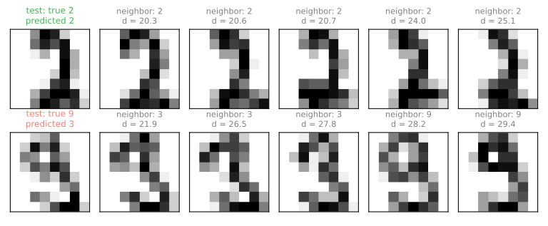
Esta é a grande vantagem do k-NN: toda previsão vem com a sua evidência. O 2 está cercado de 2. O 9 mal lido foi desenhado com uma laçada fina e aberta; as três imagens de treino mais próximas são 3 (a 21,9, 26,5 e 27,8) e os primeiros 9 só aparecem em 4º e 5º lugar (28,2 e 29,4). Com \(k = 5\) a votação ainda daria 3 contra 2. Não há peso nem coeficiente para interpretar: dá para mostrar a um usuário os cinco casos mais parecidos e deixá-lo julgar.
Simulação: deslocar um dígito um pixel. Pegue o 2 de teste #0 e desloque a imagem uma coluna para a direita (a coluna que entra fica em branco). A que distância a imagem deslocada fica da original? Compare com a distância dos vizinhos acima (20,3). O que o 3-NN prevê para ela? Depois desloque todas as imagens de teste 1 e 2 pixels, para os dois lados, e meça a acurácia.
Solução
def shift(X, dx):
    """Desloca imagens 8x8 dx colunas (dx > 0: para a direita); o que entra fica em branco."""
    imgs = X.reshape(-1, 8, 8)
    out = np.zeros_like(imgs)
    if dx > 0:
        out[:, :, dx:] = imgs[:, :, :-dx]
    elif dx < 0:
        out[:, :, :dx] = imgs[:, :, -dx:]
    else:
        out = imgs.copy()
    return out.reshape(len(X), 64)

moved = shift(Xd_test[[0]], 1)
dist, idx = knn_d.kneighbors(moved)
print(f"distância até a própria imagem original: {np.linalg.norm(moved - Xd_test[[0]]):.1f}")
print(f"previsão: {knn_d.predict(moved)[0]} · vizinhos {yd_train[idx[0]]} a distâncias {dist[0].round(1)}")
for dx in [-2, -1, 0, 1, 2]:
    print(f"deslocamento {dx:+d}: acurácia {knn_d.score(shift(Xd_test, dx), yd_test):.3f}")
distância até a própria imagem original: 50.7
previsão: 0 · vizinhos [9 0 0] a distâncias [50.4 50.4 50.4]
deslocamento -2: acurácia 0.162
deslocamento -1: acurácia 0.598
deslocamento +0: acurácia 0.987
deslocamento +1: acurácia 0.604
deslocamento +2: acurácia 0.133
Para os nossos olhos, o 2 deslocado é o mesmo 2. Para a distância, ele está a 50,7 da própria imagem original, mais que o dobro da distância até outros 2 escritos por outras pessoas (20,3). A distância compara pixel com pixel: um traço que andou uma coluna cai em pixels que antes estavam em branco e a imagem vira "outra coisa". Os vizinhos mais próximos dela estão todos a 50,4, quase tão longe quanto a própria original: nada no treino se parece com um 2 deslocado e o 3-NN prevê 0. No conjunto de teste inteiro, deslocar um pixel derruba a acurácia de 98,7% para cerca de 60%; dois pixels, para cerca de 15%, perto de chutar. O k-NN só é tão bom quanto a distância que você dá a ele. Aqui ela não sabe nada de forma; os remédios são acrescentar ao treino cópias deslocadas das imagens (Sua vez) ou usar atributos que não mudam com o deslocamento, como os que as redes neurais aprendem.
Passo 8 — acrescentar atributos de ruído
Preveja. Acrescente às 64 colunas reais colunas de ruído puro, na mesma faixa de 0 a 16. Com 64 colunas de ruído (tantas quanto as reais), a acurácia cai muito ou pouco? E com 1.024?
rng = np.random.default_rng(0)
for n_noise in [0, 64, 256, 1024]:
    noise = rng.uniform(0, 16, size=(len(Xd), n_noise))      # "pixels" falsos, na mesma faixa dos reais
    Xn = np.hstack([Xd, noise])
    a, b, c, d = train_test_split(Xn, yd, test_size=0.25, stratify=yd, random_state=0)
    acc = KNeighborsClassifier(n_neighbors=3).fit(a, c).score(b, d)
    print(f"{n_noise:5d} colunas de ruído ({Xn.shape[1]:4d} no total): acurácia {acc:.3f}")
    0 colunas de ruído (  64 no total): acurácia 0.987
   64 colunas de ruído ( 128 no total): acurácia 0.960
  256 colunas de ruído ( 320 no total): acurácia 0.842
 1024 colunas de ruído (1088 no total): acurácia 0.582
As colunas de ruído parecem pixels, mas não carregam informação nenhuma. Com tantos pixels falsos quanto reais, a acurácia cai de 98,7% para 96,0%; com 1.024 deles, para 58,2%. As imagens não mudaram e os 64 pixels reais continuam lá; eles simplesmente perdem a votação dentro da distância, em que toda coluna conta igual. Esta é a maldição da dimensionalidade na sua forma mais prática: antes de culpar o k-NN, pergunte quantas colunas de fato importam.
Simulação: o tamanho do ruído. Mantenha 1.024 colunas de ruído, mas sorteie-as em faixas menores: de 0 a 16, de 0 a 4 e de 0 a 1. Para cada faixa, meça a acurácia do 3-NN sem escalonamento e com StandardScaler num pipeline. O que prejudica o k-NN: o número de colunas de ruído ou quanto elas somam à distância?
Solução
rng = np.random.default_rng(1)
for high in [16, 4, 1]:
    noise = rng.uniform(0, high, size=(len(Xd), 1024))     # 1024 colunas de ruído, de 0 a high
    a, b, c, d = train_test_split(np.hstack([Xd, noise]), yd, test_size=0.25, stratify=yd, random_state=0)
    raw = KNeighborsClassifier(n_neighbors=3).fit(a, c).score(b, d)
    std = make_pipeline(StandardScaler(), KNeighborsClassifier(n_neighbors=3)).fit(a, c).score(b, d)
    print(f"ruído de 0 a {high:2d}: bruto {raw:.3f} · padronizado {std:.3f}")
ruído de 0 a 16: bruto 0.544 · padronizado 0.429
ruído de 0 a  4: bruto 0.982 · padronizado 0.424
ruído de 0 a  1: bruto 0.987 · padronizado 0.462
Sem escalonamento, as mesmas 1.024 colunas quase não atrapalham quando são pequenas: com ruído de 0 a 1, o 3-NN volta aos 98,7% das imagens limpas, porque cada coluna falsa soma muito pouco à distância e os pixels reais decidem. (Com ruído de 0 a 16 ele faz 54,4% e não os 58,2% do passo 8, porque o ruído sorteado é outro.) O que prejudica é quanto as colunas inúteis pesam na distância, não quantas são. O StandardScaler desfaz isso: ele dá a toda coluna o mesmo peso, inclusive às inúteis, e a acurácia fica abaixo de 50% nas três faixas. Escalonar é necessário para que as unidades não decidam por acidente, mas não separa colunas úteis de inúteis. Isso é trabalho seu: escolher os atributos antes de medir distâncias.
Para fechar a aula. Em uma frase cada: (1) por que um 2 deslocado de um pixel foi lido como 0? (2) Por que padronizar ajudou nos vinhos e não ajudou nos dígitos? (3) No passo 8, o que prejudicou o k-NN: o número de colunas de ruído ou quanto elas pesam na distância?
Sua vez (avançado)
Para casa, com mais tempo:
- Pesos. Repita o passo 5 com
KNeighborsClassifier(n_neighbors=k, weights='distance'). A acurácia de treino fica em 1,000 para todo \(k\)? Por quê? (Dica: qual é o peso de um vizinho a distância 0?) - Escolher \(k\) para os dígitos. O passo 6 usou \(k = 3\) sem justificativa. Separe uma divisão de validação de dentro de
Xd_train, avalie \(k\) ímpar de 1 a 15 commetric='euclidean'e commetric='manhattan', escolha o melhor par e só então meça o teste, uma vez. - Ensinar o deslocamento. Acrescente ao treino cópias de cada imagem deslocadas um pixel para a esquerda e para a direita (use a função
shiftda simulação do passo 7; os rótulos se repetem). Refaça a medida de acurácia nas imagens de teste deslocadas. Quanto volta? Quanto custa, em linhas guardadas e em distâncias por previsão? - Resgate com PCA. Na versão com 1.024 colunas de ruído de 0 a 16, coloque
PCA(n_components=30)antes do k-NN num pipeline. Quanto da acurácia perdida volta? Por que a PCA conseguiria separar os pixels reais do ruído aqui? (Redução de Dimensionalidade) - Regressão. Com
load_diabetes(return_X_y=True), compare oKNeighborsRegressor(escalonado, \(k\) escolhido numa divisão de validação) com aLinearRegressionnum hold-out, usando \(R^2\). Qual vence? Isso bate com o que a seção da maldição da dimensionalidade preveria com 10 atributos e 442 linhas?
Referências
- Fix, E.; Hodges, J. L. "Discriminatory Analysis. Nonparametric Discrimination: Consistency Properties." Relatório 4, USAF School of Aviation Medicine (1951); reimpresso em International Statistical Review 57 (1989). DOI
- Cover, T.; Hart, P. "Nearest Neighbor Pattern Classification." IEEE Trans. Inf. Theory 13 (1967) — o limite "no máximo o dobro do erro de Bayes". DOI
- Beyer, K.; Goldstein, J.; Ramakrishnan, R.; Shaft, U. "When Is 'Nearest Neighbor' Meaningful?" Database Theory — ICDT'99, LNCS 1540, Springer (1999): 217–235 — concentração das distâncias em dimensões altas. DOI
Quiz
O quiz cobre a abordagem fundamental.