Regressão Logística
Esta aula abre o bloco de classificação do curso. Até aqui o alvo era um número (um preço, uma nota); daqui em diante é uma categoria: sobreviveu ou não, spam ou não, qual de três espécies. O primeiro modelo é a regressão logística (Cox, 1958; sua curva remonta a Verhulst, 1838). Apesar do nome, ela é um classificador: o primeiro modelo padrão para qualquer problema de classificação e presença constante na análise de crédito e na medicina. É também a porta de entrada para as redes neurais, onde um único neurônio é uma regressão logística.
Você já conhece todas as peças que a compõem: o escore linear da regressão linear e o laço do gradiente descendente. As novidades são uma função (a sigmoide), uma perda (a entropia cruzada) e um jeito de ler coeficientes (as chances ou odds). Todos os números abaixo saem do código desta página; cada figura, de um script curto que fica ao lado dela.
A aula segue um único pipeline em cinco etapas, desenhado abaixo: 1. por que não a reta, o que dá errado quando a regressão linear classifica; 2. escore → probabilidade, a sigmoide, a fronteira de decisão e as chances; 3. perda e treino, a entropia cruzada e o gradiente descendente; 4. além da reta, fronteiras curvas e mais de duas classes; 5. probabilidade → rótulo, o limiar e quando usar o modelo. Cada etapa leva à sua seção; nos slides, uma faixa embaixo mostra em que etapa você está.
- Por que não a retauma reta falha ao classificar
- Escore → probabilidadesigmoide, fronteira de decisão, chances (odds)
- Perda e treinoentropia cruzada, não erro quadrático; gradiente descendente
- Além da retafronteiras curvas; muitas classes com softmax
- Probabilidade → rótuloo limiar é uma escolha; quando usar o modelo
Slides
Clique nos slides e use as setas ← → para navegar; F abre em tela cheia e Esc mostra todos os slides. Abrir os slides numa aba nova
O que é classificação
Um problema de classificação tem um alvo \(y\) que assume valores num conjunto finito de classes:
| classes | exemplos | |
|---|---|---|
| binária | 2, codificadas como 0 e 1 | aprovado/reprovado, fraude/legítima, maligno/benigno, sobreviveu/morreu |
| multiclasse | \(k > 2\) | espécie de íris, dígito de 0 a 9, categoria de produto |
Quase todo classificador trabalha em dois passos. Primeiro calcula, para cada exemplo, um escore ou uma probabilidade para cada classe ("esta passageira sobrevive com probabilidade 0,94"). Depois um limiar transforma esse número em rótulo ("0,94 ≥ 0,5, então: sobreviveu"). Não confunda as duas etapas: quase toda esta aula trata da primeira; a última seção trata da segunda. O jeito mais simples de avaliar os rótulos é a acurácia, a fração de acertos. Ela basta para esta aula; suas armadilhas e as métricas mais adequadas são o assunto de Métricas de Classificação.
Por que não uma reta?
Etapa 1. A primeira tentativa óbvia: codificar as classes como 0 e 1, ajustar uma regressão linear e chamar de "aprovado" tudo o que a reta colocar acima de 0,5. Considere 23 estudantes, as horas que estudaram e se foram aprovados. Depois acrescente cinco estudantes que estudaram muito e foram aprovados, como seria de esperar. (Um detalhe do código: o LogisticRegression do scikit-learn acrescenta por padrão a penalidade L2 que você viu no Ridge; C=np.inf a desliga, de modo que ajustamos exatamente o modelo desta aula. A penalidade e o ajuste do C voltam na aula de validação cruzada.)
import numpy as np
from sklearn.linear_model import LinearRegression, LogisticRegression

hours = np.arange(1, 12.5, 0.5)                    # 23 estudantes: 1; 1,5; ...; 12 horas de estudo
passed = np.array([0] * 11 + [1, 0] + [1] * 10)    # reprovam até 6 h, zona mista, aprovam a partir de 7,5 h
far = np.array([25, 30, 35, 40, 45])               # cinco estudantes que estudaram muito e passaram

for label, h, y in [('23 estudantes', hours, passed),
                    ('+ 5 aprovados distantes', np.r_[hours, far], np.r_[passed, [1] * 5])]:
    X = h.reshape(-1, 1)
    line = LinearRegression().fit(X, y)
    logit = LogisticRegression(C=np.inf).fit(X, y)     # C=np.inf: o modelo puro, sem penalidade
    out = line.predict(X)
    print(f"{label}:")
    print(f"  reta      saídas de {out.min():.2f} a {out.max():.2f}, cruza 0.5 em "
          f"{(0.5 - line.intercept_) / line.coef_[0]:.2f} h, erros: {((out >= 0.5) != y).sum()}")
    print(f"  logística cruza 0.5 em {-logit.intercept_[0] / logit.coef_[0, 0]:.2f} h, "
          f"erros: {(logit.predict(X) != y).sum()}")
23 estudantes:
  reta      saídas de -0.23 a 1.18, cruza 0.5 em 6.67 h, erros: 2
  logística cruza 0.5 em 6.75 h, erros: 2
+ 5 aprovados distantes:
  reta      saídas de 0.31 a 1.39, cruza 0.5 em 8.66 h, erros: 4
  logística cruza 0.5 em 6.75 h, erros: 2
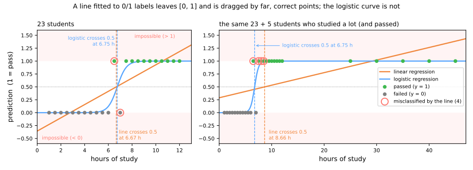
Dois problemas, ambos visíveis na figura:
- A reta sai de [0, 1]. Ela prevê −0,23 para quem estudou uma hora e 1,18 para quem estudou doze. Nenhum dos dois é uma probabilidade; a pergunta "quão seguro está o modelo?" fica sem resposta.
- Pontos corretos a prejudicam. Os cinco estudantes distantes são casos fáceis, rotulados exatamente como qualquer um esperaria. Mas os mínimos quadrados querem a reta perto deles, o que achata a inclinação e arrasta o cruzamento de 0,5 de 6,67 h para 8,66 h. Três estudantes que estudaram de 7,5 a 8,5 horas e passaram agora são chamados de "reprovados" (quem reprovou com 7 horas passa a ser acertado por acaso). Os erros vão de 2 para 4 por causa de dados que concordavam com o modelo.
A curva logística cruza 0,5 em 6,75 horas nos dois casos e comete os mesmos 2 erros (quem passou com 6,5 horas e quem reprovou com 7, que nenhum limiar sobre as horas consegue acertar). Um estudante com 45 horas está na parte plana da curva, com probabilidade ≈ 1, onde não há mais nada a corrigir; por isso quase não puxa o ajuste. Toda a ideia está nessa parte plana.
Da reta à probabilidade
Etapa 2. A regressão logística mantém o escore linear que você conhece,
e o passa pela função sigmoide (ou logística), que espreme qualquer número real no intervalo (0, 1):
Vale memorizar três valores: \(\sigma(0) = 0{,}5\); \(z\) grande e positivo dá \(\hat p \to 1\); \(z\) grande e negativo dá \(\hat p \to 0\). A previsão é classe 1 quando \(\hat p \geq 0{,}5\), o que é o mesmo que \(z \geq 0\).
À mão, depois com o scikit-learn
Ajustado nos 23 estudantes, o modelo é \(w = 2{,}619\) por hora e \(b = -17{,}681\). Três estudantes novos:
| horas \(x\) | \(z = 2{,}619x - 17{,}681\) | \(e^{-z}\) | \(\hat p = 1/(1+e^{-z})\) | classe |
|---|---|---|---|---|
| 4 | −7,205 | 1346 | 0,001 | 0 (reprova) |
| 6 | −1,967 | 7,149 | 0,123 | 0 (reprova) |
| 7,5 | 1,962 | 0,1406 | 0,877 | 1 (aprova) |
Uma calculadora basta. Agora o mesmo com a biblioteca. decision_function devolve o escore \(z\), predict_proba as probabilidades de cada classe (a coluna 1 é a classe 1) e predict o rótulo:
def sigmoid(z):
    return 1 / (1 + np.exp(-z))

model = LogisticRegression(C=np.inf).fit(hours.reshape(-1, 1), passed)
print(f"w = {model.coef_[0, 0]:.3f}   b = {model.intercept_[0]:.3f}")

new = np.array([[4.0], [6.0], [7.5]])          # três estudantes novos
z = model.decision_function(new)               # o escore w*x + b
print("z            ", z.round(3))
print("sigmoid(z)   ", sigmoid(z).round(3))
print("predict_proba", model.predict_proba(new)[:, 1].round(3))
print("predict      ", model.predict(new))
w = 2.619   b = -17.681
z             [-7.203 -1.965  1.964]
sigmoid(z)    [0.001 0.123 0.877]
predict_proba [0.001 0.123 0.877]
predict       [0 0 1]
As probabilidades batem com a tabela em três casas decimais (a terceira casa de \(z\) difere um pouco porque o código usa \(w\) e \(b\) sem arredondar). E predict_proba é literalmente sigmoid(decision_function): não há mais nada dentro do modelo.
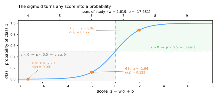
O eixo de cima da figura é a mesma curva lida em horas: o ponto mais íngreme, \(\hat p = 0{,}5\), fica em \(-b/w = 6{,}75\) horas; bastam menos de duas horas para cada lado para ir de "quase certamente reprova" a "quase certamente aprova". A inclinação é dada por \(w\): um \(w\) maior faz uma transição mais abrupta.
A fronteira de decisão é uma reta
Com dois atributos, o escore é \(z = w_1x_1 + w_2x_2 + b\); o conjunto dos pontos onde \(z = 0\) (probabilidade exatamente 0,5) é uma reta e, com \(d\) atributos, um hiperplano. Isso faz da regressão logística um classificador linear: não importa como as probabilidades variam, a fronteira entre "prever 0" e "prever 1" é plana. Considere 200 pontos em duas classes:
from sklearn.datasets import make_blobs

X2, y2 = make_blobs(n_samples=200, centers=[[-1, -0.5], [1, 1]], cluster_std=1.0, random_state=0)
clf = LogisticRegression(C=np.inf).fit(X2, y2)
w, b = clf.coef_[0], clf.intercept_[0]
print(f"w = {w.round(3)}   b = {b:.3f}   |w| = {np.linalg.norm(w):.3f}")

# afastar-se da fronteira na direção de w, partindo de dois pontos diferentes dela
u = w / np.linalg.norm(w)                              # vetor unitário perpendicular à fronteira
for start in [np.array([-b / w[0], 0.0]), np.array([0.0, -b / w[1]])]:
    pts = start + np.outer([-1, 0, 0.5, 1, 2], u)      # distâncias -1, 0, 0.5, 1, 2
    print(clf.predict_proba(pts)[:, 1].round(3))
print(sigmoid(np.linalg.norm(w) * np.array([-1, 0, 0.5, 1, 2])).round(3))
w = [1.832 1.371]   b = -0.266   |w| = 2.288
[0.092 0.5   0.758 0.908 0.99 ]
[0.092 0.5   0.758 0.908 0.99 ]
[0.092 0.5   0.758 0.908 0.99 ]
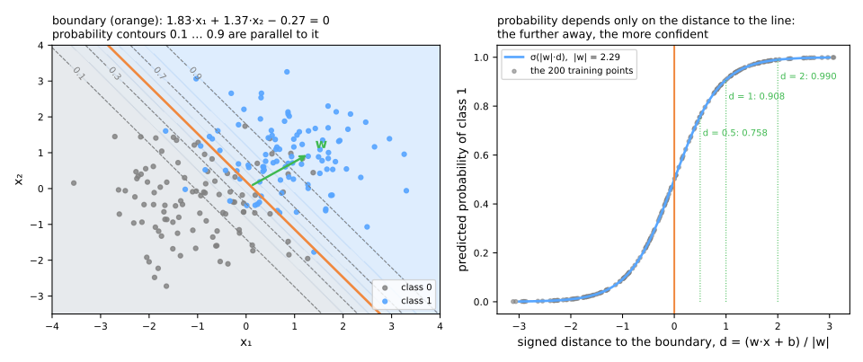
Dois pontos de partida diferentes sobre a reta, as mesmas cinco distâncias, as mesmas cinco probabilidades: 0,092, 0,5, 0,758, 0,908, 0,99. A probabilidade depende apenas da distância com sinal \(d\) até a fronteira, por meio de \(\hat p = \sigma(\lVert w\rVert\, d)\), que é a terceira linha da saída. Geometricamente:
- o vetor \(w\) é perpendicular à fronteira e aponta para a classe 1 (a seta verde);
- os contornos de mesma probabilidade são retas paralelas à fronteira;
- \(\lVert w\rVert\) define a rapidez com que a confiança cresce com a distância. Aqui \(\lVert w\rVert = 2{,}29\), então a uma unidade da reta o modelo já está 90,8% seguro.
Chances (odds) e interpretabilidade
Na regressão linear, cada coeficiente tem uma leitura direta: uma unidade a mais de \(x_j\) soma \(w_j\) à previsão. Na regressão logística, \(w_j\) também é somado ao escore \(z\), mas o que acontece com a probabilidade? A resposta aparece quando a probabilidade é escrita de outro jeito: como chance.
A chance (odds) de um evento é a probabilidade de ele acontecer dividida pela probabilidade de não acontecer, \(p/(1-p)\). É a linguagem das apostas:
| probabilidade \(p\) | chance \(p/(1-p)\) | em palavras |
|---|---|---|
| 0,75 | 0,75 / 0,25 = 3 | "3 para 1": em 4 casos, 3 a favor e 1 contra |
| 0,5 | 0,5 / 0,5 = 1 | "1 para 1": tanto faz |
| 0,2 | 0,2 / 0,8 = 0,25 | "1 para 4": em 5 casos, 1 a favor e 4 contra |
A probabilidade vai de 0 a 1; a chance vai de 0 a infinito e vale 1 quando \(p = 0{,}5\).
Agora a ligação com o modelo. A probabilidade prevista é \(\hat p = \sigma(z) = 1/(1+e^{-z})\), então a probabilidade do contrário é \(1 - \hat p = e^{-z}/(1+e^{-z})\). Ao dividir uma pela outra, o denominador \(1 + e^{-z}\) some:
A chance que o modelo prevê é simplesmente \(e^{z}\). Lida da direita para a esquerda, a mesma igualdade diz que o escore \(z\) é o log da chance, o logito (logit, nome cunhado por Berkson em 1944, por analogia com o "probit" de Bliss). O modelo é linear no log da chance, não na probabilidade.
Um exemplo com números. Tome um modelo de um único atributo com \(w = 0{,}8\) e \(b = -4\). Para cada valor de \(x\), a tabela calcula, da esquerda para a direita: o escore \(z = wx + b\); a probabilidade prevista \(\hat p = \sigma(z)\), com a mesma sigmoide de antes; a chance \(\hat p/(1-\hat p)\); por fim, \(e^{z}\) para conferir a conta acima.
| \(x\) | escore \(z = 0{,}8x - 4\) | probabilidade \(\hat p = \sigma(z)\) | chance \(\hat p/(1-\hat p)\) | \(e^{z}\) |
|---|---|---|---|---|
| 4 | −0,8 | 0,310 | 0,449 | 0,449 |
| 5 | 0,0 | 0,500 | 1,000 | 1,000 |
| 6 | +0,8 | 0,690 | 2,226 | 2,226 |
As duas últimas colunas coincidem, como prometido. Agora compare as linhas. Cada unidade a mais de \(x\) soma 0,8 ao escore; como a chance é \(e^{z}\), somar 0,8 ao expoente multiplica a chance por \(e^{0{,}8} = 2{,}226\). Por isso a coluna das chances vai de 0,449 a 1,000 e depois a 2,226, cada valor 2,226 vezes o anterior. Em geral:
A probabilidade, por sua vez, não segue regra fixa. Ela sobe 19 pontos de \(x=4\) para \(x=5\) e outros 19 de 5 para 6, mas isso é coincidência da simetria em torno de 0,5; mais longe do centro, os saltos mudam de tamanho (o modelo das horas, logo abaixo, mostra isso).
Eis a leitura correta de um coeficiente logístico: uma unidade a mais de \(x_j\) multiplica a chance por \(e^{w_j}\), em qualquer ponto da curva, mantidos os outros atributos fixos. A variação em probabilidade depende de onde você parte: máxima perto de \(p = 0{,}5\), desprezível nas caudas. A mesma verificação no modelo das horas:
print(f"e^w = {np.exp(model.coef_[0, 0]):.3f}")
odds = lambda p: p / (1 - p)
p = model.predict_proba([[5.0], [6.0], [7.0]])[:, 1]
print("p       ", p.round(3))
print("chances ", odds(p).round(3))
print("razões  ", (odds(p)[1:] / odds(p)[:-1]).round(3))
Cada hora a mais de estudo multiplica a chance de aprovação por 13,7. Em probabilidade, isso é +11 pontos de 5 para 6 horas, mas +54 pontos de 6 para 7. A razão de chances \(e^{w}\) é o número que médicos e analistas de crédito citam; é também o motivo de a regressão logística seguir em uso em domínios regulados (Explicabilidade). Dois cuidados vêm da regressão linear: a leitura supõe os outros atributos fixos; além disso, só é justo comparar coeficientes quando os atributos estão em escalas comparáveis (você fará isso com atributos padronizados no lab).
A perda: entropia cruzada
Etapa 3. Para ajustar \(w\) e \(b\) precisamos de um número que meça o quanto as probabilidades estão erradas. O princípio é a máxima verossimilhança: escolher os parâmetros sob os quais os rótulos que de fato observamos sejam os mais prováveis possível. A probabilidade que o modelo dá ao que aconteceu com o exemplo \(i\) é \(\hat p_i\) se \(y_i = 1\) e \(1 - \hat p_i\) se \(y_i = 0\). Multiplicando sobre os exemplos, tomando o log (que transforma o produto em soma) e trocando o sinal para que menor seja melhor, obtém-se a log loss ou entropia cruzada binária:
Para cada exemplo, só um dos dois termos não se anula. Cada termo se lê: menos o log da probabilidade que o modelo deu à verdade.
À mão
Quatro previsões, duas de cada classe:
| \(i\) | \(y\) | \(\hat p\) | probabilidade dada à verdade | \(-\ln(\cdot)\) |
|---|---|---|---|---|
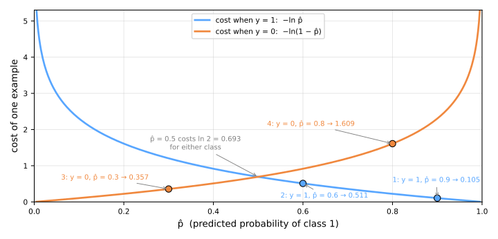
| 1 | 1 | 0,9 | 0,9 | 0,105 |
| 2 | 1 | 0,6 | 0,6 | 0,511 |
| 3 | 0 | 0,3 | 0,7 | 0,357 |
| 4 | 0 | 0,8 | 0,2 | 1,609 |
A média é \((0{,}105 + 0{,}511 + 0{,}357 + 1{,}609)/4 = 0{,}646\). A biblioteca concorda:
from sklearn.metrics import log_loss

y_true = np.array([1, 1, 0, 0])
p_hat = np.array([0.9, 0.6, 0.3, 0.8])
terms = -(y_true * np.log(p_hat) + (1 - y_true) * np.log(1 - p_hat))
print(terms.round(3), f"média = {terms.mean():.3f}")
print(f"log_loss = {log_loss(y_true, p_hat):.3f}")
O ponto 4 é o único erro, cometido com alta confiança (0,8 para a classe errada). Sozinho ele contribui com 1,609 do total de 2,582, 62%. Um acerto tímido (ponto 2, 0,6) custa 0,511; um acerto confiante (ponto 1) custa 0,105. A perda recompensa acertar e ser honesto sobre o grau de certeza. Dois valores de referência: um modelo que sempre diz 0,5 obtém \(\ln 2 = 0{,}693\); um modelo perfeito, 0.
A figura desenha os dois termos da soma como curvas em função de \(\hat p\), com os quatro pontos da tabela sobre elas. Para um exemplo da classe 1 só a curva azul conta, \(-\ln \hat p\); para a classe 0, só a laranja, \(-\ln(1 - \hat p)\). Cada curva vale 0 na ponta certa e cresce sem limite na ponta errada: passar de 0,8 para 0,99 na classe errada leva o custo do ponto 4 de 1,609 para 4,6. As duas curvas se cruzam em \(\hat p = 0{,}5\), onde qualquer classe custa \(\ln 2\). A perda média é só a altura média dos pontos.
Por que não o erro quadrático?
A regressão linear usava o erro quadrático. Por que não usar aqui \((y - \hat p)^2\), que também é pequeno quando \(\hat p\) acerta e grande quando erra? Porque, combinado com a sigmoide, ele falha em três pontos. A figura resume os três; em seguida, cada painel é explicado com números.
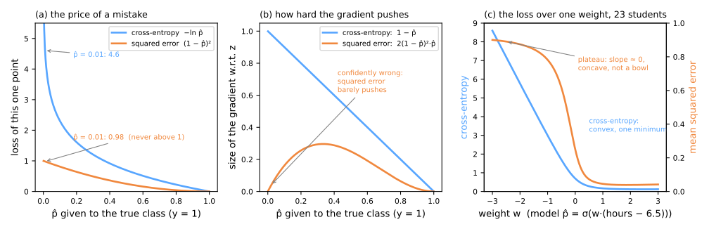
Os painéis (a) e (b) olham para um único exemplo da classe 1 (\(y = 1\)) e variam a probabilidade \(\hat p\) que o modelo dá a ele; para a classe 0 tudo é simétrico. O painel (c) olha para a perda média de um conjunto inteiro.
(a) O preço de um erro. Quanto custa esse exemplo em cada perda:
| \(\hat p\) dada à classe certa | situação | erro quadrático \((1-\hat p)^2\) | entropia cruzada \(-\ln \hat p\) |
|---|---|---|---|
| 0,9 | acerto confiante | 0,010 | 0,105 |
| 0,5 | em cima do muro | 0,250 | 0,693 |
| 0,1 | erro | 0,810 | 2,303 |
| 0,01 | erro grave | 0,980 | 4,605 |
| 0,001 | erro gravíssimo | 0,998 | 6,908 |
O erro quadrático nunca passa de 1: para ele, errar com \(\hat p = 0{,}1\) ou com \(\hat p = 0{,}001\) custa quase o mesmo (0,810 contra 0,998). A entropia cruzada separa bem os dois casos (2,303 contra 6,908): cada fator 10 a mais de confiança no erro acrescenta 2,3 à perda.
(b) O empurrão do gradiente. Este é o problema principal. O gradiente descendente corrige um exemplo mexendo no escore \(z\) dele. A força dessa correção é a derivada da perda \(L\) em relação a \(z\). Pela regra da cadeia, ela tem dois fatores:
O segundo fator é a inclinação da sigmoide. Ele é quase zero nas partes planas da curva, ou seja, sempre que o modelo está muito confiante, certo ou errado. Para \(y = 1\):
- erro quadrático: \(\partial L/\partial \hat p = -2(1-\hat p)\), logo \(\partial L/\partial z = -2(1-\hat p)\cdot \hat p(1-\hat p)\). A inclinação da sigmoide continua multiplicando e, perto de \(\hat p = 0\), apaga o gradiente;
- entropia cruzada: \(\partial L/\partial \hat p = -1/\hat p\), logo \(\partial L/\partial z = -\frac{1}{\hat p}\cdot \hat p(1-\hat p) = -(1-\hat p) = \hat p - y\). O \(1/\hat p\) cancela o \(\hat p\) da inclinação da sigmoide.
Em números (o sinal negativo só indica "aumente \(z\)"; o que importa é o tamanho):
| \(\hat p\) dada à classe certa | inclinação da sigmoide \(\hat p(1-\hat p)\) | \(\partial L/\partial z\), erro quadrático | \(\partial L/\partial z\), entropia cruzada |
|---|---|---|---|
| 0,5 | 0,25 | −0,250 | −0,500 |
| 0,1 | 0,09 | −0,162 | −0,900 |
| 0,01 | 0,0099 | −0,0196 | −0,990 |
| 0,001 | 0,001 | −0,0020 | −0,999 |
Leia a coluna do erro quadrático de cima para baixo: quanto pior o erro, mais fraco o empurrão. Em \(\hat p = 0{,}001\) ele é 500 vezes mais fraco que o da entropia cruzada. Os exemplos que o modelo mais precisa corrigir são justamente os que o erro quadrático ignora. Na entropia cruzada acontece o contrário: o empurrão cresce com o erro, até o máximo de 1. Guarde esse fator \(\hat p(1-\hat p)\), que nunca passa de 0,25: nas redes neurais, multiplicado camada após camada, é ele que apaga os gradientes de redes profundas com sigmoide. A última linha, conferida em código:
y1, p1 = 1, 0.001                                           # classe verdadeira 1, o modelo diz 0,1%
print(f"d(MSE)/dz = {2 * (p1 - y1) * p1 * (1 - p1):.4f}   d(CE)/dz = {p1 - y1:.4f}")
(c) O formato da perda. Agora a perda média nos 23 estudantes, em função de um peso. Para caber num gráfico, o modelo tem um único parâmetro: \(\hat p = \sigma(w\,(\text{horas} - 6{,}5))\), com as horas centralizadas em 6,5, perto da fronteira real de 6,75 h. Com \(w > 0\), mais horas dão mais probabilidade de aprovação: a direção certa. Com \(w < 0\), o modelo aposta que quem estuda mais reprova; é a direção errada e quase todo estudante vira um erro confiante.
x_c = hours - 6.5                                          # centraliza as horas em 6,5
for wt in [-3, -1, 0, 1, 3]:
    p = sigmoid(wt * x_c)
    mse = np.mean((passed - p) ** 2)
    ce = -np.mean(passed * np.log(p) + (1 - passed) * np.log(1 - p))
    print(f"w = {wt:+d}   MSE = {mse:.3f}   entropia cruzada = {ce:.3f}")
w = -3   MSE = 0.900   entropia cruzada = 8.597
w = -1   MSE = 0.782   entropia cruzada = 2.992
w = +0   MSE = 0.250   entropia cruzada = 0.693
w = +1   MSE = 0.045   entropia cruzada = 0.166
w = +3   MSE = 0.042   entropia cruzada = 0.118
Imagine o gradiente descendente começando em \(w = -3\). Com o erro quadrático, a perda quase não muda de \(w = -3\) para \(w = -1\) (de 0,900 para 0,782): o terreno é um platô, a inclinação é pequena e os passos também. É o efeito (b) somado sobre os 23 estudantes, todos errados com confiança. Com a entropia cruzada, o mesmo trecho desce de 8,597 para 2,992: a inclinação é forte e aponta claramente para o lado certo. Há ainda uma garantia. Na regressão logística, a entropia cruzada é convexa em \(w\) e \(b\): um só vale, sem mínimos locais onde ficar preso. O erro quadrático não é convexo (no platô a curva se dobra para baixo) e não oferece essa garantia.
O simulador coloca as duas perdas lado a lado em outro conjunto pequeno. Mexa em \(w\) e \(b\) e observe o painel da direita:
Treino por gradiente descendente
Não há fórmula fechada para o mínimo de \(J\), como havia para os mínimos quadrados, então descemos até ele. A derivada é curta. Para um exemplo, a regra da cadeia através de \(\hat p = \sigma(z)\) e \(\sigma'(z) = \sigma(z)(1-\sigma(z))\) dá
e como \(z = w^\top x + b\), a derivada em relação a \(w_j\) só multiplica por \(x_j\). Tirando a média sobre os exemplos:
É o mesmo formato do gradiente da regressão linear, \(X^\top(\text{previsão} - y)\), com \(\hat p = \sigma(Xw + b)\) no lugar de \(Xw\) (o fator 2 de lá vem do quadrado). Cada exemplo contribui na proporção do erro da sua probabilidade. Cada iteração do laço tem quatro etapas, com os nomes que elas vão receber nas redes neurais:
- forward: calcular as probabilidades, \(\hat p = \sigma(Xw + b)\);
- perda: medir a entropia cruzada \(J\);
- backward: calcular os gradientes \(\nabla_w J = \frac{1}{n}X^\top(\hat p - y)\) e \(\partial J/\partial b\);
- atualização: \(w \leftarrow w - \eta\,\nabla_w J\) e \(b \leftarrow b - \eta\,\partial J/\partial b\).
O laço de gradiente descendente da aula anterior, nos 200 pontos acima:
w_gd, b_gd, eta = np.zeros(2), 0.0, 0.5
for it in range(2001):
    p = sigmoid(X2 @ w_gd + b_gd)
    if it in (0, 10, 100, 1000, 2000):
        loss = -np.mean(y2 * np.log(p) + (1 - y2) * np.log(1 - p))
        print(f"iter {it:4d}  perda {loss:.4f}  w {w_gd.round(4)}  b {b_gd:.4f}")
    w_gd -= eta * X2.T @ (p - y2) / len(y2)            # o gradiente acima
    b_gd -= eta * np.mean(p - y2)
print(f"sklearn           w {clf.coef_[0].round(4)}  b {clf.intercept_[0]:.4f}")
iter    0  perda 0.6931  w [0. 0.]  b 0.0000
iter   10  perda 0.3391  w [1.0142 0.6968]  b -0.0484
iter  100  perda 0.2956  w [1.7785 1.3219]  b -0.2455
iter 1000  perda 0.2955  w [1.8315 1.3718]  b -0.2663
iter 2000  perda 0.2955  w [1.8315 1.3718]  b -0.2663
sklearn           w [1.8317 1.3713]  b -0.2661
A perda começa em \(\ln 2 = 0{,}6931\) (todos os pesos zero significam \(\hat p = 0{,}5\) para todo mundo), cai rápido nos 10 primeiros passos e para de mudar em 0,2955 antes da iteração 1000. Os pesos concordam com os do scikit-learn a menos de 0,0005; a diferença vem de o scikit-learn parar assim que suas melhorias ficam abaixo da tolerância (tol=1e-4). O scikit-learn não usa este laço simples (seu solver padrão, lbfgs, também usa informação de curvatura e converge em poucos passos, 7 neste exemplo), mas minimiza a mesma função e chega ao mesmo lugar, porque uma função convexa tem um único fundo. A versão estocástica também existe: assim como o SGDRegressor da aula anterior ajusta a regressão linear com SGD, o SGDClassifier(loss='log_loss', penalty=None) ajusta esta mesma regressão logística.
Fronteiras curvas: construa os atributos
Etapa 4. Até aqui toda fronteira foi uma reta: o conjunto dos pontos em que \(z = w_1x_1 + w_2x_2 + b = 0\). Muitos problemas não se separam com uma reta. O exemplo clássico são os círculos: uma classe forma um círculo pequeno no centro e a outra, um círculo maior em volta dele. Qualquer reta deixa pedaços do círculo externo dos dois lados.
A saída não exige um modelo novo. A regressão logística é linear nos atributos que recebe, que não precisam ser as medidas originais. Se, em vez de \(x_1\) e \(x_2\), ela receber \(x_1^2\) e \(x_2^2\), o escore passa a ser
e a fronteira \(z = 0\) vira \(w_1 x_1^2 + w_2 x_2^2 = -b\). Com \(w_1\) e \(w_2\) negativos e parecidos, isso é um círculo. É a mesma ideia dos atributos polinomiais que permitiram à regressão linear ajustar uma parábola: o modelo continua linear nos atributos, mas a fronteira aparece curva quando desenhada nas medidas originais.
Em dados: 400 pontos, 200 no círculo interno (classe 1) e 200 no externo (classe 0), com o raio interno igual à metade do externo e um pouco de ruído. 30% dos pontos (120) ficam separados para teste:
from sklearn.datasets import make_circles
from sklearn.model_selection import train_test_split

X, y = make_circles(n_samples=400, noise=0.15, factor=0.5, random_state=0)   # classe 1 = círculo interno
X_a, X_b, y_a, y_b = train_test_split(X, y, test_size=0.3, stratify=y, random_state=0)

flat = LogisticRegression(C=np.inf).fit(X_a, y_a)                  # atributos x1, x2
circle = LogisticRegression(C=np.inf).fit(X_a ** 2, y_a)           # atributos x1², x2²
print(f"x1, x2      teste {flat.score(X_b, y_b):.3f}")
print(f"x1², x2²    teste {circle.score(X_b ** 2, y_b):.3f}   w = {circle.coef_[0].round(2)}   b = {circle.intercept_[0]:.2f}")
Com \(x_1\) e \(x_2\), a reta acerta 40,0% do teste, pior que uma moeda: nenhuma reta separa um círculo de outro que o envolve (ficar abaixo de 50% é acaso de uma amostra de 120 pontos). Com \(x_1^2\) e \(x_2^2\), acerta 100%. Os dois pesos saíram quase iguais (−16,83 e −16,00), ou seja, o modelo descobriu sozinho que a fronteira é redonda: \(z = 0\) quando \(16{,}8\,x_1^2 + 16{,}0\,x_2^2 = 9{,}70\), um círculo de raio \(\sqrt{9{,}70/16{,}4} \approx 0{,}77\), entre o círculo interno (raio 0,5) e o externo (raio 1). Dentro dele \(z > 0\): o modelo prevê a classe 1.
Quando a forma não é óbvia. Nos círculos, sabíamos de antemão que a fronteira era redonda. Em geral não sabemos. A alternativa é gerar de uma vez todos os produtos das medidas até certo grau, com o PolynomialFeatures. Com duas medidas e grau 3, são 9 atributos: \(x_1, x_2, x_1^2, x_1x_2, x_2^2, x_1^3, x_1^2x_2, x_1x_2^2, x_2^3\). A fronteira \(z = 0\) pode então ser qualquer curva de grau 3. O teste abaixo compara a reta com essa versão em dois formatos: os círculos e as luas, duas meias-luas encaixadas uma na outra (também 400 pontos, 30% para teste):
from sklearn.datasets import make_moons
from sklearn.pipeline import make_pipeline
from sklearn.preprocessing import PolynomialFeatures, StandardScaler

for name, (X, y) in [('luas', make_moons(n_samples=400, noise=0.2, random_state=0)),
                     ('círculos', make_circles(n_samples=400, noise=0.15, factor=0.5, random_state=0))]:
    X_a, X_b, y_a, y_b = train_test_split(X, y, test_size=0.3, stratify=y, random_state=0)
    plain = make_pipeline(StandardScaler(), LogisticRegression(C=np.inf)).fit(X_a, y_a)
    poly = make_pipeline(PolynomialFeatures(degree=3, include_bias=False), StandardScaler(),
                         LogisticRegression(C=np.inf, max_iter=5000)).fit(X_a, y_a)
    print(f"{name:8s} simples: teste {plain.score(X_b, y_b):.3f}   "
          f"grau 3 ({poly[0].n_output_features_} atributos): teste {poly.score(X_b, y_b):.3f}")
luas     simples: teste 0.917   grau 3 (9 atributos): teste 0.958
círculos simples: teste 0.400   grau 3 (9 atributos): teste 0.958
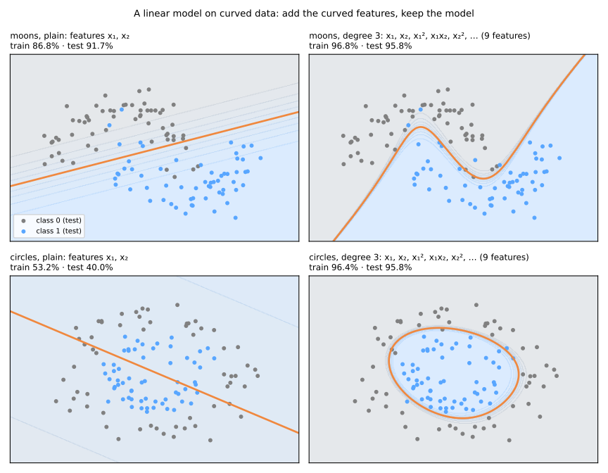
Nas luas, a reta já vai razoavelmente bem (91,7%), porque só as pontas das meias-luas se encaixam; a curva de grau 3 contorna as pontas e chega a 95,8%. Nos círculos, os 9 atributos genéricos também resolvem o problema (95,8%), mas ficam abaixo dos 2 atributos certos (100%). Quando se conhece a forma, construir o atributo certo vale mais que gerar muitos.
Repare no StandardScaler depois do PolynomialFeatures. Nas luas, \(x_1\) vai de −1,35 a 2,4, mas \(x_1^3\) vai de −2,4 a 13,8. Atributos em escalas tão diferentes esticam a paisagem da perda e os solvers baseados em gradiente descem devagar por ela. Padronizar depois de expandir põe todos os atributos na mesma escala.
O modelo continua sendo uma regressão logística comum, só que com 9 atributos: entropia cruzada, convexidade e gradiente valem como antes. Há dois preços. O primeiro é a interpretação: a leitura "uma unidade a mais de \(x_j\), mantidos os outros fixos" perde o sentido, porque \(x_1^2\) não muda sem que \(x_1\) mude junto. O segundo é o sobreajuste: mais atributos dão mais capacidade de sobreajustar, como você viu na aula anterior. Quando nem os polinômios capturam a forma da fronteira, entram os modelos que a encontram sozinhos: na próxima aula, o k-NN; depois, as árvores e as redes neurais.
Multiclasse: softmax
Para \(k\) classes o modelo aprende um vetor de pesos e um intercepto por classe, o que dá \(k\) escores \(z_c = w_c^\top x + b_c\). O softmax transforma os escores em probabilidades positivas que somam 1:
À mão
Três escores \(z = (2{,}0;\ 1{,}0;\ 0{,}1)\):
| classe | \(z_c\) | \(e^{z_c}\) | \(\hat p_c = e^{z_c} / 11{,}212\) |
|---|---|---|---|
| A | 2,0 | 7,389 | 0,659 |
| B | 1,0 | 2,718 | 0,242 |
| C | 0,1 | 1,105 | 0,099 |
| soma | 11,212 | 1,000 |
O maior escore vence, mas não leva tudo: uma diferença de 1 no escore é um fator \(e \approx 2{,}7\) na probabilidade. Somar a mesma constante a todos os escores não muda nada (multiplica numerador e denominador pelo mesmo \(e^c\)). É por isso que o código subtrai o maior escore antes de exponenciar, para evitar estouro numérico. Com duas classes, o softmax é a sigmoide: \(e^{z_1}/(e^{z_0}+e^{z_1}) = \sigma(z_1 - z_0)\).
Com o scikit-learn, no wine
O conjunto wine: 178 vinhos de três cultivares (variedades de uva) da mesma região italiana, cada um descrito por 13 medidas químicas. Para manter o exemplo pequeno, usamos duas delas, o teor alcoólico e os flavonoides. O LogisticRegression passa sozinho para o softmax quando \(y\) tem mais de duas classes:
from sklearn.datasets import load_wine

def softmax(z):
    e = np.exp(z - z.max(axis=1, keepdims=True))       # subtrair o máximo: mesmo resultado, sem estouro
    return e / e.sum(axis=1, keepdims=True)

wine = load_wine()
cols = [wine.feature_names.index(c) for c in ['alcohol', 'flavanoids']]
Xw, yw = wine.data[:, cols], wine.target
wine_model = make_pipeline(StandardScaler(), LogisticRegression(C=np.inf)).fit(Xw, yw)
print(wine.target_names, "coef_:", wine_model[-1].coef_.shape, "intercept_:", wine_model[-1].intercept_.shape)

picks = [0, 100, 133]                                  # um vinho de cada cultivar
z = wine_model.decision_function(Xw[picks])            # 3 escores por vinho
print("true cultivar", yw[picks])
print("scores\n", z.round(2))
print("softmax\n", softmax(z).round(3))
print("predict_proba\n", wine_model.predict_proba(Xw[picks]).round(3))
print("predict      ", wine_model.predict(Xw[picks]))
P = wine_model.predict_proba(Xw)
print(f"rows sum to 1: {np.allclose(P.sum(axis=1), 1)}   "
      f"max |predict_proba - softmax|: {np.abs(P - softmax(wine_model.decision_function(Xw))).max()}")
['class_0' 'class_1' 'class_2'] coef_: (3, 2) intercept_: (3,)
true cultivar [0 1 2]
scores
 [[ 6.47 -0.22 -6.25]
 [-0.29  5.32 -5.02]
 [-3.11  1.56  1.55]]
softmax
 [[0.999 0.001 0.   ]
 [0.004 0.996 0.   ]
 [0.005 0.502 0.493]]
predict_proba
 [[0.999 0.001 0.   ]
 [0.004 0.996 0.   ]
 [0.005 0.502 0.493]]
predict       [0 1 1]
rows sum to 1: True   max |predict_proba - softmax|: 0.0
coef_ tem formato (3, 2): uma linha de 2 pesos por cultivar, mais 3 interceptos. O predict_proba é exatamente softmax(decision_function) e toda linha soma 1. Os três vinhos são instrutivos. O vinho 0 é da cultivar 0, com 0,999: fácil. O vinho 100 é da cultivar 1, com 0,996. O vinho 133 pertence à cultivar 2, mas seus escores para as cultivares 1 e 2 estão quase empatados (1,56 e 1,55); o modelo o divide em 0,502 / 0,493 e o predict erra, por um fio. As probabilidades dizem quão ambíguo ele é, coisa que um rótulo sozinho não diz.
A perda é a mesma entropia cruzada, \(-\ln \hat p_{\text{classe verdadeira}}\), em média. O vinho 0 custa \(-\ln 0{,}999 \approx 0{,}001\); o vinho 133, cuja cultivar verdadeira recebeu só 0,493, custa \(-\ln 0{,}493 \approx 0{,}706\), setecentas vezes mais. Essa construção exata (escores lineares, softmax, entropia cruzada) é a camada de saída de praticamente todo classificador neural, inclusive dos modelos de linguagem que escolhem o próximo token entre dezenas de milhares.
Das probabilidades aos rótulos: o limiar
Etapa 5. predict é predict_proba mais um limiar de 0,5 (para duas classes; para várias, a classe de maior probabilidade). O 0,5 é uma escolha, não parte do modelo. Nos 200 pontos de antes, movê-lo troca um tipo de erro pelo outro:
p_hat = clf.predict_proba(X2)[:, 1]
print("predict == (p >= 0.5):", np.array_equal(clf.predict(X2), (p_hat >= 0.5).astype(int)))
for t in [0.2, 0.5, 0.8]:
    pred = (p_hat >= t).astype(int)
    print(f"limiar {t}: classe 1 prevista {pred.sum():3d} vezes · classe 1 perdida: "
          f"{((pred == 0) & (y2 == 1)).sum():2d} · alarmes falsos: {((pred == 1) & (y2 == 0)).sum():2d}"
          f" · acurácia {np.mean(pred == y2):.3f}")
predict == (p >= 0.5): True
limiar 0.2: classe 1 prevista 131 vezes · classe 1 perdida:  1 · alarmes falsos: 32 · acurácia 0.835
limiar 0.5: classe 1 prevista  97 vezes · classe 1 perdida: 12 · alarmes falsos:  9 · acurácia 0.895
limiar 0.8: classe 1 prevista  76 vezes · classe 1 perdida: 31 · alarmes falsos:  7 · acurácia 0.810
Baixar o limiar para 0,2 quase não perde ponto da classe 1 (1 em vez de 12) e paga com 32 alarmes falsos em vez de 9; subi-lo para 0,8 faz o contrário. A acurácia é melhor em 0,5 aqui, mas a acurácia conta os dois erros como igualmente ruins. Quando deixar passar um câncer é pior que um alarme falso ou quando a classe positiva é rara, esse é o critério errado e o limiar deve se mover. Como medir os dois tipos de erro e escolher o limiar é o assunto de Métricas de Classificação e de Curvas ROC & PR. A contribuição da regressão logística é fornecer probabilidades às quais vale a pena aplicar um limiar.
Perfil prático
| Pontos fortes | rápida para treinar e para prever; perda convexa (a mesma resposta toda vez, sem sorte de inicialização); probabilidades em geral razoáveis sem ajuste; interpretável por razões de chances; uma baseline forte que escala para milhões de linhas |
| Fraquezas | fronteira linear (curvas exigem atributos construídos); interações entre atributos precisam ser acrescentadas à mão; converge devagar com atributos não escalonados; a leitura dos coeficientes de atributos correlacionados é instável, mesmo quando as previsões vão bem |
| Cuidado com | avisos de max_iter costumam indicar atributos não escalonados; colunas one-hot para todas as categorias ao lado de um intercepto deixam cada coeficiente sem sentido sozinho (descarte uma categoria de referência); razões de chances não são razões de probabilidades |
| Recorra a ela quando | você precisa de uma baseline sólida e explicável; as probabilidades importam (risco, triagem, ranqueamento); os atributos são informativos individualmente |
Lab: prevendo a sobrevivência no Titanic
A lista de passageiros do Titanic da aula de pré-processamento, agora com uma pergunta: quem sobreviveu? O lab aplica tudo o que foi visto acima a dados reais e bagunçados: um pipeline com imputação, codificação e escalonamento; probabilidades conferidas à mão; coeficientes lidos como razões de chances; e uma estimativa honesta da acurácia em passageiros que o modelo nunca viu. O modelo é a regressão logística pura desta aula (C=np.inf), então não há nada para ajustar: dividimos os dados uma vez em treino (ajustar e estudar o modelo) e teste (reportar, uma vez, no fim).
Como fazer este lab em aula (cerca de 60 min, em duplas)
- Abra o notebook do lab no Colab e salve uma cópia no seu Drive (Arquivo → Salvar uma cópia no Drive) antes de editar. Rode as células em ordem, numa mesma sessão.
- Cada passo começa com um Preveja: responda com a dupla antes de rodar a célula. Errar a previsão é o que torna o resultado memorável.
- Depois de rodar, compare com a saída e a leitura desta página. Toda saída aqui é exatamente o que o código imprime.
- As Simulações pedem que vocês escrevam um pequeno experimento em Python: mudar uma entrada do modelo e observar o que acontece com a saída. Nada de conta à mão. A solução fica recolhida logo abaixo: tente antes de abrir.
- Ritmo sugerido: passos 1 a 4 em 20 min; passos 5 a 7 em 25 min; passo 8 e discussão final em 15 min. Sua vez fica para casa.
Passo 1 — carregar e olhar
Preveja. A taxa de sobrevivência geral fica acima ou abaixo de 50%? Quem sobreviveu mais: as mulheres da 3ª classe ou os homens da 1ª?
import numpy as np
import pandas as pd

url = "https://raw.githubusercontent.com/hsandmann/biblio/refs/heads/main/ml/aula04/titanic/train.csv"
df = pd.read_csv(url)
print(df.shape)
print(f"taxa de sobrevivência: {df['Survived'].mean():.3f}")
print(df.pivot_table(index='Sex', columns='Pclass', values='Survived', aggfunc='mean').round(3))
print("faltantes:", df[['Age', 'Embarked', 'Cabin']].isna().sum().to_dict())
(891, 12)
taxa de sobrevivência: 0.384
Pclass      1      2      3
Sex
female  0.968  0.921  0.500
male    0.369  0.157  0.135
faltantes: {'Age': 177, 'Embarked': 2, 'Cabin': 687}
891 passageiros, 38,4% sobreviveram. A tabela, com a taxa de sobrevivência por sexo e classe da passagem, já conta quase toda a história: 96,8% das mulheres da primeira classe sobreviveram, contra 13,5% dos homens da terceira. Duas coisas a guardar para depois. Sexo e classe importam e interagem: para as mulheres, ir da 2ª para a 3ª classe custa 42 pontos (0,921 → 0,500); para os homens, 2 pontos (0,157 → 0,135). Uma regressão logística só com as colunas Sex e Pclass não consegue representar isso sozinha (ver Sua vez). E Age falta para 177 passageiros, Embarked para 2, Cabin para 687; vamos imputar as duas primeiras e deixar Cabin de fora.
Passo 2 — treino e teste
Preveja. Por que separar o conjunto de teste agora, antes de montar qualquer modelo? Por que não deixar isso para o fim?
from sklearn.model_selection import train_test_split

features = ['Pclass', 'Sex', 'Age', 'SibSp', 'Parch', 'Fare', 'Embarked']
X, y = df[features], df['Survived']
X_train, X_test, y_train, y_test = train_test_split(X, y, test_size=0.2, stratify=y, random_state=42)
print(len(X_train), len(X_test))
print(f"taxa de sobrevivência: treino {y_train.mean():.3f} · teste {y_test.mean():.3f}")
Dos passageiros, 80% (712) vão para o treino e 20% (179) para o conjunto de teste, que não é tocado de novo até o passo 8. stratify mantém a taxa de sobrevivência em 38% nas duas partes. Os atributos são as sete colunas cruas; Name, Ticket, Cabin e PassengerId ficam de fora. Não há conjunto de validação porque não há nada a escolher: o modelo puro não tem hiperparâmetro para ajustar. (Quando tiver, separe uma parte das linhas de treino para validação ou use a validação cruzada, que vem mais adiante no curso.)
Passo 3 — uma baseline
Preveja. Um "modelo" que responde sempre "não sobreviveu", sem olhar o passageiro, acerta mais ou menos da metade das vezes? Por quê?
from sklearn.dummy import DummyClassifier

dummy = DummyClassifier(strategy='most_frequent').fit(X_train, y_train)
print(f"sempre 'não sobreviveu': acurácia de treino {dummy.score(X_train, y_train):.3f}")
Um "modelo" que ignora o passageiro e sempre responde a classe majoritária ("não sobreviveu") acerta 61,7% das vezes no treino. Esse é o piso. Qualquer acurácia que reportarmos só significa algo em comparação com ele; no passo 8, os dois são medidos no conjunto de teste.
Passo 4 — o pipeline
Preveja. Pclass vale 1, 2 ou 3. Por que tratá-la como categoria (uma coluna one-hot para cada classe) e não como um número?
from sklearn.compose import ColumnTransformer
from sklearn.impute import SimpleImputer
from sklearn.linear_model import LogisticRegression
from sklearn.pipeline import make_pipeline
from sklearn.preprocessing import OneHotEncoder, StandardScaler

numeric = ['Age', 'SibSp', 'Parch', 'Fare']
categorical = ['Pclass', 'Sex', 'Embarked']

preprocess = ColumnTransformer([
    ('num', make_pipeline(SimpleImputer(strategy='median'), StandardScaler()), numeric),
    ('cat', make_pipeline(SimpleImputer(strategy='most_frequent'),
                          OneHotEncoder(drop='first')), categorical)])
model = make_pipeline(preprocess, LogisticRegression(C=np.inf, max_iter=1000))   # C=np.inf: sem penalidade
model.fit(X_train, y_train)

enc = model[0].named_transformers_['cat'][-1]
print("categorias de referência (descartadas):", {c: cats[0] for c, cats in zip(categorical, enc.categories_)})
print(f"{model[-1].coef_.size} coeficientes · acurácia de treino {model.score(X_train, y_train):.3f}")
categorias de referência (descartadas): {'Pclass': 1, 'Sex': 'female', 'Embarked': 'C'}
9 coeficientes · acurácia de treino 0.809
O ColumnTransformer manda cada coluna para o seu tratamento: os números recebem a mediana no lugar dos faltantes e depois são padronizados; as categorias recebem o valor mais frequente e passam por one-hot. Pclass é tratada como categoria, sem supor que a 2ª classe fica exatamente "no meio" entre a 1ª e a 3ª. Tudo é ajustado só nas linhas de treino, dentro do pipeline.
Por que drop='first'. Se o codificador mantivesse uma coluna por categoria, todo passageiro teria exatamente um 1 entre Pclass_1, Pclass_2 e Pclass_3: as três colunas somariam sempre 1, exatamente como a coluna constante que o intercepto multiplica. Somar 5 aos três pesos de classe e subtrair 5 do intercepto daria então as mesmas previsões; o modelo teria infinitos conjuntos de pesos igualmente bons e nenhum coeficiente one-hot isolado significaria nada. Descartar a primeira categoria de cada variável elimina essa redundância. As categorias descartadas são a referência, impressa na primeira linha: uma mulher da primeira classe que embarcou em Cherbourg. Todo coeficiente one-hot restante se lê em relação a essa referência (passo 7). Sobram 9 coeficientes: 4 numéricos, 2 de classe, 1 de sexo e 2 do porto.
O modelo acerta 80,9% dos passageiros de treino, contra 61,7% da baseline. A acurácia de treino é otimista (esses passageiros foram usados para ajustar os pesos), mas com 9 coeficientes para 712 passageiros há pouco espaço para sobreajuste; o passo 8 vai medir o quanto ela era otimista.
Passo 5 — probabilidades para dois passageiros
Preveja. Olhando a tabela do passo 1: um homem da 3ª classe e uma mulher da 1ª classe. Quem recebe probabilidade alta e quem recebe baixa?
passengers = pd.DataFrame({'Pclass': [3, 1], 'Sex': ['male', 'female'], 'Age': [25, 30],
                           'SibSp': [0, 1], 'Parch': [0, 0], 'Fare': [8.05, 80.0],
                           'Embarked': ['S', 'C']})
print(model.predict_proba(passengers).round(3))
print(model.predict(passengers))
Dois passageiros inventados: um homem de 25 anos viajando sozinho na terceira classe, com passagem de 8 libras, embarcado em Southampton; e uma mulher de 30 anos na primeira classe com o marido, passagem de 80 libras, embarcada em Cherbourg. Cada linha de predict_proba é (não sobreviveu, sobreviveu) e soma 1. O modelo dá a ele 9,3% e a ela 94,2%, coerente com a tabela do passo 1.
Simulação: o efeito da idade. Tome um passageiro da 2ª classe que viaja com os pais (Parch = 2) e um irmão (SibSp = 1), passagem de 30 libras, embarcado em Southampton. Mude só a idade (2, 8, 15, 25, 40 e 60 anos), primeiro para um menino e depois para uma menina. Observe a probabilidade prevista. Depois confira nas linhas de treino quantas crianças de até 12 anos da 2ª classe sobreviveram.
Solução
ages = [2, 8, 15, 25, 40, 60]
print("idade  ", ages)
for sex in ['male', 'female']:
    people = pd.DataFrame({'Pclass': 2, 'Sex': sex, 'Age': ages, 'SibSp': 1, 'Parch': 2,
                           'Fare': 30.0, 'Embarked': 'S'})
    print(f"{sex:7s}", model.predict_proba(people)[:, 1].round(3))

train = df.loc[X_train.index]                        # só as linhas de treino
kids = train[(train['Age'] <= 12) & (train['Pclass'] == 2)]
print(kids.groupby('Sex')['Survived'].agg(['mean', 'size']))
idade   [2, 8, 15, 25, 40, 60]
male    [0.38  0.326 0.268 0.198 0.12  0.059]
female  [0.9   0.876 0.843 0.784 0.667 0.477]
        mean  size
Sex
female   1.0     7
male     1.0     8
Para o modelo, a idade tem o mesmo efeito em todo mundo: a probabilidade cai suavemente com os anos, para meninos e para meninas. O menino de 8 anos recebe só 32,6%. Nos dados de treino, porém, as 15 crianças de até 12 anos da 2ª classe sobreviveram todas, meninos inclusive. A regra "mulheres e crianças primeiro" é uma interação entre idade e sexo: ser criança muda muito o destino de um menino e pouco o de uma menina. Uma regressão logística só a representa se alguém construir o atributo que a descreve; o exercício 1 de Sua vez faz isso para outra interação, entre sexo e classe.
Passo 6 — a probabilidade do homem, à mão
Preveja. Olhando os coeficientes que vão aparecer, qual atributo você espera que mais derrube o escore do homem?
names = model[0].get_feature_names_out()
w, b = model[-1].coef_[0], model[-1].intercept_[0]
x_man = model[0].transform(passengers)[0]            # o homem da 3ª classe, depois do pré-processamento
print(pd.DataFrame({'x': x_man, 'w': w, 'w*x': w * x_man}, index=names).round(3))
z = b + (w * x_man).sum()
print(f"z = {b:.3f} + {(w * x_man).sum():.3f} = {z:.3f}   sigmoid(z) = {1 / (1 + np.exp(-z)):.3f}")
                     x      w    w*x
num__Age        -0.350 -0.513  0.180
num__SibSp      -0.465 -0.267  0.124
num__Parch      -0.466 -0.072  0.034
num__Fare       -0.495  0.108 -0.053
cat__Pclass_2    0.000 -0.987 -0.000
cat__Pclass_3    1.000 -2.239 -2.239
cat__Sex_male    1.000 -2.685 -2.685
cat__Embarked_Q  0.000  0.320  0.000
cat__Embarked_S  1.000 -0.417 -0.417
z = 2.782 + -5.057 = -2.275   sigmoid(z) = 0.093
Eis o modelo inteiro, por dentro. A coluna x é o que chega ao classificador: os quatro números padronizados (25 anos está 0,350 desvio-padrão abaixo da média do treino, daí \(-0{,}350\)) e um 1 na coluna de cada categoria não referência a que ele pertence: terceira classe, homem, Southampton. Multiplique pelos pesos, some tudo e acrescente o intercepto: \(z = -2{,}275\). Então \(\sigma(-2{,}275) = 0{,}093\), os 9,3% do passo 5.
Com uma categoria de referência, o intercepto ganha leitura própria: \(b = 2{,}782\) é o log das chances do passageiro de referência, uma mulher da primeira classe embarcada em Cherbourg, com idade, família e tarifa médias, cuja probabilidade é \(\sigma(2{,}782) = 0{,}942\). A partir dela, ser homem tira 2,685 do escore, a terceira classe tira 2,239 e Southampton, 0,417. A juventude dele ajuda um pouco (+0,180, porque o coeficiente da idade é negativo e ele é mais novo que a média); viajar sozinho também ajuda (+0,124).
Simulação: um atributo por vez. Parta do homem da 3ª classe e transforme-o, um passo de cada vez, na passageira de referência: primeiro mude o sexo para female, depois a classe para 1, depois o porto para C. A cada passo, imprima o escore \(z\) (model.decision_function) e a probabilidade. Quanto \(z\) muda em cada passo? E a probabilidade?
Solução
step = passengers.iloc[[0]].copy()                  # começa no homem da 3ª classe
z_old, p_old = model.decision_function(step)[0], model.predict_proba(step)[0, 1]
print(f"{'início':22s} z = {z_old:+.3f}             p = {p_old:.3f}")
for col, val in [('Sex', 'female'), ('Pclass', 1), ('Embarked', 'C')]:
    step[col] = val
    z, p = model.decision_function(step)[0], model.predict_proba(step)[0, 1]
    print(f"{col + ' -> ' + str(val):22s} z = {z:+.3f} ({z - z_old:+.3f})   p = {p:.3f} ({p - p_old:+.3f})")
    z_old, p_old = z, p
início                 z = -2.275             p = 0.093
Sex -> female          z = +0.410 (+2.685)   p = 0.601 (+0.508)
Pclass -> 1            z = +2.649 (+2.239)   p = 0.934 (+0.333)
Embarked -> C          z = +3.066 (+0.417)   p = 0.955 (+0.022)
Cada mudança soma ao escore exatamente o seu coeficiente (2,685, 2,239 e 0,417, os números da tabela acima), não importa de onde se parta. A probabilidade não se comporta assim: a mesma mudança vale muito perto de 0,5 e quase nada perto de 1. Trocar o porto soma 0,417 ao escore, mas só 2 pontos à probabilidade, porque ela já estava em 0,934, na parte plana da sigmoide.
Passo 7 — coeficientes como razões de chances
Preveja. O coeficiente de Age é negativo. Então, com o resto fixo, um passageiro mais velho tem chance maior ou menor de sobreviver? A razão de chances \(e^{\text{coef}}\) dele fica acima ou abaixo de 1?
coef = pd.Series(w, index=names)
print(pd.DataFrame({'coef': coef, 'e^coef': np.exp(coef)}).round(3))
sd = model[0].named_transformers_['num'][-1].scale_
print("um desvio-padrão:", ", ".join(f"{c} {s:.1f}" for c, s in zip(numeric, sd)))
                  coef  e^coef
num__Age        -0.513   0.599
num__SibSp      -0.267   0.765
num__Parch      -0.072   0.931
num__Fare        0.108   1.114
cat__Pclass_2   -0.987   0.373
cat__Pclass_3   -2.239   0.107
cat__Sex_male   -2.685   0.068
cat__Embarked_Q  0.320   1.377
cat__Embarked_S -0.417   0.659
um desvio-padrão: Age 13.0, SibSp 1.1, Parch 0.8, Fare 48.0
Atributos numéricos estão padronizados, então cada coeficiente vale por um desvio-padrão, impresso na última linha. Idade: \(e^{-0{,}513} = 0{,}599\), ou seja, 13,0 anos a mais multiplicam a chance de sobreviver por 0,599 (uma chance cerca de 40% menor), com sexo, classe, tarifa e o resto fixos. Tarifa: um desvio-padrão (48,0 libras) multiplica a chance por 1,114.
Atributos one-hot comparam sua categoria com a categoria de referência da mesma variável, com todo o resto fixo. Sex_male = -2.685: a chance de sobreviver de um homem é \(e^{-2{,}685} = 0{,}068\) vez a de uma mulher com a mesma classe, idade, família, tarifa e porto. Pclass_3 = -2.239: a chance de um passageiro da terceira classe é 0,107 vez a de um passageiro idêntico da primeira; a de um da segunda classe, 0,373 vez. Embarked_S: a chance de quem embarcou em Southampton é 0,659 vez a de quem embarcou em Cherbourg. Para ler uma comparação no sentido contrário, troque o sinal (e inverta a razão de chances); para comparar duas categorias que não são a referência, subtraia seus coeficientes:
print(f"mulher vs homem:  chance x {np.exp(-coef['cat__Sex_male']):.2f}")
print(f"1ª vs 3ª classe:  chance x {np.exp(-coef['cat__Pclass_3']):.2f}")
print(f"2ª vs 3ª classe:  chance x {np.exp(coef['cat__Pclass_2'] - coef['cat__Pclass_3']):.2f}")
A chance de sobreviver de uma mulher é 14,7 vezes a de um homem com a mesma classe, idade, tarifa, família e porto. A de um passageiro da primeira classe é 9,4 vezes a de um passageiro idêntico da terceira; a de um da segunda, 3,5 vezes. Esses são os números a reportar. A escolha da categoria de referência é uma questão de apresentação: outra escolha muda os coeficientes, mas nenhuma previsão. E razão de chances não é razão de probabilidades: 14,7 vezes a chance não é 14,7 vezes a probabilidade, que não pode passar de 1.
Simulação: a razão de chances é a mesma para todo mundo. Tome três passageiros diferentes (o homem da 3ª classe, um homem de 30 anos da 1ª classe e o menino da simulação do passo 5). Para cada um, calcule com predict_proba a probabilidade como mulher e como homem, mantendo todo o resto. Compare a razão entre as probabilidades e a razão entre as chances.
Solução
odds = lambda p: p / (1 - p)
people = pd.DataFrame({'Pclass': [3, 1, 2], 'Sex': 'male', 'Age': [25, 30, 8], 'SibSp': [0, 1, 1],
                       'Parch': [0, 0, 2], 'Fare': [8.05, 80.0, 30.0], 'Embarked': ['S', 'C', 'S']})
for i in range(len(people)):
    one = people.iloc[[i]]
    p_f = model.predict_proba(one.assign(Sex='female'))[0, 1]
    p_m = model.predict_proba(one.assign(Sex='male'))[0, 1]
    print(f"p mulher {p_f:.3f} · p homem {p_m:.3f} · razão de probabilidades {p_f / p_m:5.2f}"
          f" · razão de chances {odds(p_f) / odds(p_m):.2f}")
p mulher 0.601 · p homem 0.093 · razão de probabilidades  6.45 · razão de chances 14.66
p mulher 0.942 · p homem 0.523 · razão de probabilidades  1.80 · razão de chances 14.66
p mulher 0.876 · p homem 0.326 · razão de probabilidades  2.69 · razão de chances 14.66
A razão de chances sai 14,66 para os três, exatamente o \(e^{2{,}685}\) da tabela: é o único número que descreve o efeito do sexo para qualquer passageiro. A razão de probabilidades muda de passageiro para passageiro (de 1,80 a 6,45), porque depende de onde cada um parte. Por isso se reporta a razão de chances.
Passo 8 — o único teste
Preveja. A acurácia de teste vai ficar acima ou abaixo dos 80,9% de treino? Muito ou pouco?
from sklearn.metrics import confusion_matrix

print(f"acurácia de teste {model.score(X_test, y_test):.3f} · baseline {dummy.score(X_test, y_test):.3f}")
print(confusion_matrix(y_test, model.predict(X_test), labels=[1, 0]))   # positivo primeiro
Só agora tocamos o conjunto de teste: 80,4% de acurácia contra 61,5% da baseline, perto dos 80,9% do treino; o número de treino era só um pouco otimista. A tabela 2×2 é uma primeira olhada na matriz de confusão: as linhas são a verdade (sobreviveu, morreu), as colunas a previsão, com a classe positiva primeiro: o layout padrão, [[TP, FN], [FP, TN]], que o labels=[1, 0] pede ao scikit-learn. Dos 69 sobreviventes do conjunto de teste, o modelo deixou passar 23; dos 110 que morreram, chamou 12 de sobreviventes. A acurácia mistura esses dois tipos de erro num número só; as próximas aulas os separam.
Se 80,4% decepcionar e você voltar ao passo 4 para tentar outros atributos, o conjunto de teste passa a fazer parte do seu ciclo de projeto e 80,4% deixa de significar qualquer coisa. Compare variantes numa validação separada das linhas de treino (como em Sua vez) e guarde o teste para o fim.
Simulação: mexendo no limiar. O predict usa o limiar 0,5. Nas linhas de treino (o teste já foi usado), classifique com os limiares 0,3, 0,4, 0,5, 0,6 e 0,7 e imprima, para cada um, a fração dos sobreviventes encontrados, a fração dos mortos reconhecidos e a acurácia.
Solução
p_train = model.predict_proba(X_train)[:, 1]         # no treino: o teste já foi usado
for t in [0.3, 0.4, 0.5, 0.6, 0.7]:
    pred = (p_train >= t).astype(int)
    found = pred[y_train == 1].mean()                # fração dos sobreviventes encontrados
    recog = 1 - pred[y_train == 0].mean()            # fração dos mortos reconhecidos
    print(f"limiar {t}: sobreviventes encontrados {found:.3f} · mortos reconhecidos {recog:.3f}"
          f" · acurácia {(pred == y_train).mean():.3f}")
limiar 0.3: sobreviventes encontrados 0.824 · mortos reconhecidos 0.745 · acurácia 0.775
limiar 0.4: sobreviventes encontrados 0.751 · mortos reconhecidos 0.804 · acurácia 0.784
limiar 0.5: sobreviventes encontrados 0.714 · mortos reconhecidos 0.868 · acurácia 0.809
limiar 0.6: sobreviventes encontrados 0.652 · mortos reconhecidos 0.916 · acurácia 0.815
limiar 0.7: sobreviventes encontrados 0.553 · mortos reconhecidos 0.964 · acurácia 0.806
Baixar o limiar encontra mais sobreviventes e reconhece menos mortos; subir faz o contrário. A acurácia quase não muda (de 0,775 a 0,815) e esconde essa troca. Qual limiar é o melhor depende de qual erro custa mais, não da acurácia; as duas frações têm nome (recall e especificidade) e são o assunto de Métricas de Classificação.
Para fechar a aula. Em uma frase cada: (1) o que um coeficiente da regressão logística multiplica? (2) Por que o menino da simulação do passo 5 recebeu uma probabilidade tão baixa? (3) Por que o conjunto de teste só pode ser usado uma vez?
Sua vez
Para casa, com mais tempo:
- A interação. O passo 1 mostrou que a terceira classe prejudica as mulheres muito mais que os homens. Acrescente a coluna
df['female_3rd'] = ((df['Sex'] == 'female') & (df['Pclass'] == 3)).astype(int), coloque-a emfeaturese emcategorical(comdrop='first', seu coeficiente compara 1 com 0) e refaça os passos 2 a 7. Leia a razão de chances dela em palavras. Como muda o coeficienteSex_male? Por quê? Para decidir se a coluna ajuda, dividaX_trainde novo em uma parte de treino e uma de validação e compare os dois modelos ali, não no teste. - O limiar. Nessa validação, calcule
p = model.predict_proba(X_val)[:, 1]e conte os sobreviventes perdidos e os alarmes falsos para os limiares 0,3, 0,5 e 0,7. Que limiar você usaria se perder um sobrevivente fosse três vezes pior que um alarme falso? - Por que uma categoria de referência. Monte o pipeline de novo com
OneHotEncoder()(semdrop) e ajuste-o. Depois some 5 aos três pesos dePclassemmodel[-1].coef_e subtraia 5 demodel[-1].intercept_: as probabilidades previstas emX_testmudam? O que isso diz sobre ler um único coeficiente quando toda categoria mantém sua coluna? - Do zero. Tome
Xt = model[0].transform(X_train)e rode o laço de gradiente descendente desta aula (pesos e intercepto, \(\eta = 0{,}5\)). Compare commodel[-1].coef_emodel[-1].intercept_. Depois de quantas iterações eles concordam em duas casas decimais?
Referências
- Verhulst, P.-F. "Notice sur la loi que la population suit dans son accroissement." Correspondance Mathématique et Physique 10 (1838), 113–121. texto completo
- Berkson, J. "Application of the Logistic Function to Bio-Assay." Journal of the American Statistical Association 39, n. 227 (1944): 357–365 — cunha a palavra logit. DOI
- Cox, D. R. "The Regression Analysis of Binary Sequences." JRSS B 20 (1958). DOI