Random Forest
A aula de árvores de decisão terminou no defeito crônico da árvore de decisão: ela é instável. Reajuste-a numa amostra ligeiramente diferente e a pergunta da raiz muda, as folhas mudam e muitas previsões também; as árvores têm acurácias parecidas, mas cada uma erra em linhas diferentes. A mesma aula terminou com uma pista: deixar muitas dessas árvores votarem superou cada uma delas. Esta aula transforma a pista em método. A ideia de Leo Breiman (bagging, 1996; random forests, 2001) não é combater a variância de uma árvore, mas sim fazer a média de muitas árvores diferentes e deixar que seus erros se cancelem. O resultado é um dos algoritmos mais confiáveis do aprendizado de máquina: um ponto de partida forte para dados tabulares, que quase não precisa de ajuste, estima o próprio erro de graça e treina em paralelo.
A aula primeiro mede por que a média funciona e o que a limita (a correlação entre os membros), depois constrói a floresta em dois passos (amostras bootstrap e subconjuntos aleatórios de atributos) e mede cada um. Todo número citado vem dos blocos de código ou dos scripts de figura ao lado desta página.
Como esta aula está organizada
A aula tem duas abordagens. Cada uma tem slides, texto e um lab para fazer em aula no Colab; o quiz do fim cobre a fundamental. Comece pela fundamental: a avançada parte dela.
| Abordagem fundamental | Abordagem avançada | |
|---|---|---|
| pergunta | Por que a média de muitas árvores instáveis acerta mais que qualquer uma delas e como a floresta as torna diferentes? | Onde a média para de ajudar, quais botões importam e como ler (e não ler) uma floresta |
| conteúdo | a variância de uma média, o bootstrap, bagging, a fronteira suavizada pelo voto, max_features e a descorrelação, a avaliação out-of-bag, quantas árvores | o voto de Condorcet e a correlação, o piso \(\rho\sigma^2\) medido, hiperparâmetros, importância de atributos e seus vieses, Extra-Trees, extrapolação, custo |
| lab em aula | filtro de spam: da árvore à floresta, passos 1 a 7 | ajustar, escolher o limiar e testar, passos 8 a 11 |
| ao final, você sabe | explicar por que o voto vence as árvores; dizer o que o bootstrap deixa de fora; usar o erro OOB no lugar da validação; saber quando parar de acrescentar árvores | ajustar max_features e min_samples_leaf; escolher um limiar com previsões OOB; desconfiar da importância por impureza; saber o que uma floresta não consegue fazer |
Os dois labs usam o mesmo notebook no Colab: a parte fundamental vai do passo 1 ao 7; a avançada, do 8 ao 11. Tudo roda no navegador; não é preciso baixar nada.
Abordagem fundamental
Uma pergunta guia esta parte: como uma média de modelos ruins pode ser um modelo bom? A resposta tem duas condições — membros razoáveis e erros pouco correlacionados — e a floresta é construída para atender às duas: o bootstrap dá a cada árvore uma amostra diferente e o sorteio de atributos em cada divisão as impede de começar todas pela mesma pergunta. De quebra, as linhas que cada árvore não viu dão uma validação de graça.
Esta parte segue um caminho em quatro etapas, desenhado abaixo: 1. por que a média funciona; 2. bootstrap e bagging; 3. descorrelacionar as árvores; 4. validar out-of-bag. Cada etapa leva à sua seção e, nos slides, uma faixa embaixo mostra em que etapa você está.
- Por que a média funcionaa variância de uma média e seu piso ρσ²
- Bootstrap e baggingreamostrar, crescer árvores fundas, votar
- Descorrelacionar as árvoressortear
max_featurescandidatos a cada divisão - Validar out-of-bago erro out-of-bag (OOB); quantas árvores
Slides da abordagem fundamental
Clique nos slides e use as setas ← → para navegar; F abre em tela cheia e Esc mostra todos os slides. Abrir os slides numa aba nova
1. Por que a média funciona
Etapa 1. Em 1907, Francis Galton examinou os 787 bilhetes de um concurso numa feira de gado inglesa: os visitantes pagavam seis pence para palpitar o peso de um boi depois de abatido e limpo. Os palpites individuais iam para todo lado, mas sua mediana foi 1.207 libras; o boi pesou 1.198 libras (Galton, 1907). A multidão acertou melhor que quase todos os seus membros, porque os erros individuais, apontando em direções diferentes, se cancelaram.
A aritmética por trás é curta. Tome \(n\) estimativas \(X_1, \dots, X_n\) com variância \(\sigma^2\) cada e faça a média. Se todo par tem correlação \(\rho\), então
Dois termos. O segundo encolhe quando \(n\) cresce. O primeiro, \(\rho\sigma^2\), não depende de \(n\): é a parte do erro que todos os estimadores compartilham; nenhuma quantidade de média a remove. Uma simulação confirma a fórmula. Cada estimador é um erro compartilhado mais um erro próprio, misturados de modo que a variância seja 1 e a correlação seja \(\rho\):
import numpy as np

rng = np.random.default_rng(0)
reps = 20_000                                    # repete o experimento 20.000 vezes
print(" rho    n   variance of the mean   formula")
for rho in [0.0, 0.3]:
    for n in [1, 10, 100]:
        shared = rng.normal(size=(reps, 1))      # o erro que os n estimadores compartilham
        own = rng.normal(size=(reps, n))         # o erro próprio de cada estimador
        est = np.sqrt(rho) * shared + np.sqrt(1 - rho) * own   # variância 1, correlação rho entre pares
        print(f"{rho:4.1f} {n:4d}   {est.mean(axis=1).var():20.3f}   {rho + (1 - rho) / n:7.3f}")
 rho    n   variance of the mean   formula
 0.0    1                  1.015     1.000
 0.0   10                  0.100     0.100
 0.0  100                  0.010     0.010
 0.3    1                  0.998     1.000
 0.3   10                  0.374     0.370
 0.3  100                  0.312     0.307
Com estimadores independentes (\(\rho = 0\)), a média de 10 divide a variância por 10 e a de 100, por 100. Com \(\rho = 0,3\), 10 estimadores levam a variância de 1 para 0,37 e 100 estimadores, só até 0,31: dez vezes mais trabalho por quase nada, porque o piso é \(\rho\sigma^2 = 0,3\). O painel da esquerda da figura desenha a fórmula para quatro correlações, com a simulação em pontos (script da figura):
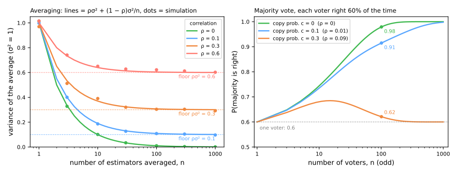
Eis tudo o que se exige de uma random forest: membros individualmente bons (\(\sigma^2\) pequeno) e o menos correlacionados possível (\(\rho\) pequeno).
2. O bootstrap: novos conjuntos de treino a partir do que você tem
Etapa 2. Para fazer a média de muitas árvores precisamos de muitos conjuntos de treino, mas só temos um. O bootstrap (Efron, 1979) fabrica novos: sorteie \(n\) linhas com reposição das \(n\) linhas que você tem. À mão, com 10 linhas:
rng = np.random.default_rng(0)
rows = np.arange(10)                             # um conjunto de treino de 10 linhas, numeradas 0..9
boot = rng.choice(rows, size=10, replace=True)   # uma amostra bootstrap: 10 sorteios com reposição
counts = np.bincount(boot, minlength=10)
print("drawn:      ", np.sort(boot))
print("times drawn:", counts)
print("left out:   ", rows[counts == 0])
A amostra tem 10 linhas, como a original, mas a linha 0 aparece três vezes, a linha 8 duas vezes e as linhas 4, 7 e 9 nenhuma vez. Uma árvore crescida nela vê uma versão levemente distorcida dos dados, com algumas linhas pesando mais e outras ausentes. É exatamente esse tipo de perturbação que faz uma árvore instável mudar.
Quantas linhas ficam de fora? Um sorteio erra uma dada linha com probabilidade \(1 - 1/n\); \(n\) sorteios independentes erram todos com probabilidade \((1 - 1/n)^n\), que tende a \(1/e\):
print("    n   (1 - 1/n)^n   simulated")
for n in [10, 100, 1000]:
    left_out = [np.mean(np.bincount(rng.integers(0, n, n), minlength=n) == 0) for _ in range(10_000)]
    print(f"{n:5d}   {(1 - 1 / n)**n:11.4f}   {np.mean(left_out):9.4f}")
print(f"limit 1/e = {np.exp(-1):.4f}")
Já com \(n = 100\), uma amostra bootstrap deixa de fora 36,6% das linhas e contém os outros 63,4%, algumas delas várias vezes. As linhas deixadas de fora serão úteis mais adiante: para a árvore que não as viu, são dados novos.
A tabela abaixo mostra seis amostras bootstrap das mesmas 10 linhas, uma por coluna: cada célula diz quantas vezes a linha foi sorteada para aquela árvore; as cinzas são as linhas deixadas de fora (script da figura):
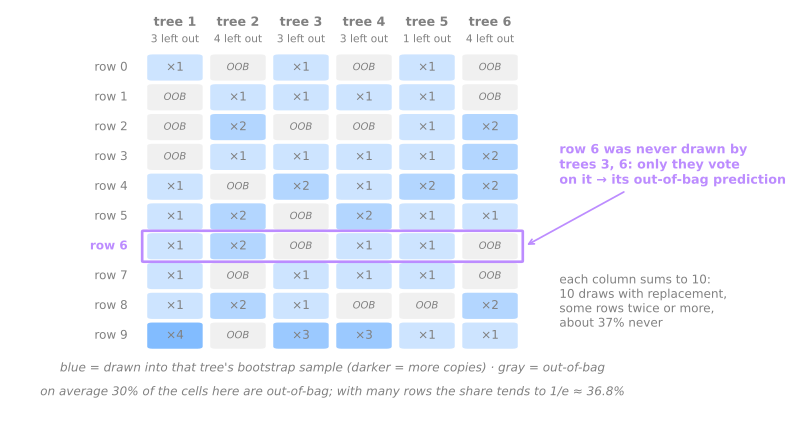
Cada coluna soma 10 sorteios; algumas linhas entram duas, três ou quatro vezes e outras nenhuma. Guarde as células cinzas: na seção 5 elas viram uma validação de graça.
3. Bagging
Bagging (bootstrap aggregating, Breiman, 1996) é a combinação das duas ideias: cresça \(B\) árvores (cada uma na sua própria amostra bootstrap, em geral até a profundidade máxima) e faça a média das previsões (regressão) ou deixe-as votar (classificação).
Variância, medida
A afirmação é que o bagging reduz a variância e deixa o viés em paz. Isso pode ser medido diretamente, porque variância diz respeito a conjuntos de treino diferentes. Sorteie 100 conjuntos de treino de 100 pontos do mesmo processo, \(y = \sin x + 0,5 \sin 3x\) mais ruído com desvio-padrão 0,3, ajuste cada modelo em cada um deles e observe as previsões em 100 pontos fixos. O viés² mede quão longe a previsão média (sobre os 100 ajustes) está da função verdadeira; a variância, quanto as 100 previsões se espalham em torno da própria média. A soma dos dois com a variância do ruído, 0,09, é o erro quadrático esperado num ponto novo:
from sklearn.ensemble import BaggingRegressor
from sklearn.tree import DecisionTreeRegressor


def truth(x):
    return np.sin(x) + 0.5 * np.sin(3 * x)


x_grid = np.linspace(0.2, 6.1, 100).reshape(-1, 1)     # 100 pontos fixos onde observamos os modelos
models = {'tree, max_depth=3': DecisionTreeRegressor(max_depth=3),
          'tree, full depth': DecisionTreeRegressor(),
          'bagging, 100 full trees': BaggingRegressor(DecisionTreeRegressor(), n_estimators=100,
                                                      random_state=0)}
preds = {name: [] for name in models}
members = []                                           # 10 das árvores do bagging, para o próximo bloco
for s in range(100):                                   # 100 conjuntos de treino do mesmo processo
    r = np.random.default_rng(s)
    x = r.uniform(0, 2 * np.pi, (100, 1))
    y = truth(x[:, 0]) + r.normal(0, 0.3, 100)         # variância do ruído 0,09
    for name, model in models.items():
        preds[name].append(model.fit(x, y).predict(x_grid))
    members.append([t.predict(x_grid) for t in models['bagging, 100 full trees'].estimators_[:10]])

print(f"{'':24s} bias²   variance   expected test MSE")
for name, P in preds.items():
    P = np.array(P)                                    # 100 conjuntos de treino × 100 pontos
    bias2 = ((P.mean(axis=0) - truth(x_grid[:, 0]))**2).mean()
    var = P.var(axis=0).mean()
    print(f"{name:24s} {bias2:.4f}  {var:.4f}     {bias2 + var + 0.09:.4f}")
                         bias²   variance   expected test MSE
tree, max_depth=3        0.0223  0.0274     0.1397
tree, full depth         0.0010  0.0883     0.1793
bagging, 100 full trees  0.0006  0.0413     0.1318
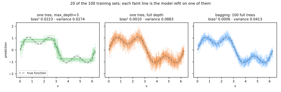
As três linhas são as três saídas para o dilema da aula de árvores de decisão:
- A árvore completa quase não tem viés (0,0010): em média, acerta. Mas cada ajuste persegue o ruído do seu próprio conjunto de treino; a variância (0,0883) é praticamente a própria variância do ruído (0,09): uma folha com um ponto prevê o ruído daquele ponto.
- Podar até profundidade 3 corta a variância para 0,0274, mas paga em viés (0,0223): oito folhas não acompanham duas ondas sobrepostas. É o compromisso viés–variância da aula de seleção de modelos, em que todo botão que baixa um sobe o outro.
- O bagging recusa o compromisso. Mantém o viés baixo das árvores completas (0,0006) e corta a variância pela metade (0,0413). Seu erro esperado, 0,1318, é o menor dos três.
Classificação: o voto suaviza a fronteira
A mesma coisa em duas dimensões, em 300 pontos ruidosos do conjunto "duas luas", avaliados em 10.000 pontos novos do mesmo processo (script da figura):
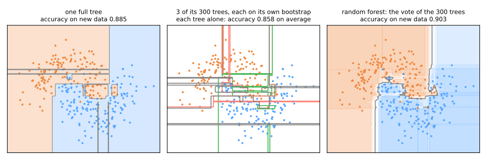
O painel do meio é o ponto central do método. Cada árvore da floresta é pior que a árvore única da esquerda (0,858 em média contra 0,885), porque viu só cerca de 63% dos pontos distintos e, em cada divisão, só uma das duas coordenadas, sorteada (a subamostragem de atributos da random forest, explicada abaixo). As árvores discordam muito sobre onde fica a fronteira; cada uma desenha as suas ilhas. Ainda assim, o voto delas, à direita, acerta 0,903, mais que qualquer uma: as ilhas ficam em lugares diferentes para árvores diferentes e perdem no voto, enquanto a forma verdadeira, que toda árvore encontra aproximadamente, sobrevive. A intensidade da cor é a fração de árvores votando em cada classe, uma confiança graduada que uma única árvore completa, com suas folhas puras, não consegue dar.
O que a média faz e o que ela não consegue fazer
O simulador abaixo cresce árvores em amostras bootstrap de 90 pontos, cada divisão considerando só uma das duas coordenadas, sorteada. O painel da esquerda mostra as árvores individuais; o da direita, o voto delas; a curva, o erro do voto em pontos novos (um conjunto de teste da mesma distribuição) à medida que árvores são acrescentadas:
Há duas coisas a notar; a segunda é a que costuma passar despercebida.
O painel da esquerda nunca melhora. Acrescente cinquenta árvores e cada uma delas continua tão trêmula quanto a primeira. O bagging não produz árvores melhores; produz uma média melhor das mesmas árvores instáveis.
A curva de erro achata. Passadas algumas dezenas de árvores, mais árvores não acrescentam nada. Não é defeito de convergência: a média ataca a variância e deixa intocados o viés e a parte da variância que as árvores compartilham, \(\rho\sigma^2\). Se a parte plana da curva está alta demais, acrescentar árvores é a única coisa que certamente não ajuda: é preciso árvores diferentes (a próxima seção), atributos melhores ou outro modelo. É também por isso que n_estimators é uma questão de orçamento, não de ajuste: mais nunca é pior, só mais lento.
4. Random forests: descorrelacionando as árvores
Etapa 3. As árvores do bagging são correlacionadas por um motivo simples: todas veem os mesmos atributos fortes. Se um atributo é de longe a melhor primeira divisão, quase toda amostra bootstrap o escolherá na raiz, as árvores começarão iguais e seus erros coincidirão. O segundo ingrediente de Breiman (2001), apoiado na ideia de subespaços aleatórios de Ho (1995, 1998) e nas árvores aleatorizadas de Amit & Geman (1997): em cada divisão, só um subconjunto aleatório de max_features atributos é elegível. O melhor deles é escolhido. Um atributo forte que não foi sorteado num nó não pode ser usado ali; outros atributos têm sua chance.
A figura mostra o mecanismo em cinco árvores e oito atributos, em que f3 é de longe a melhor primeira pergunta (script da figura):
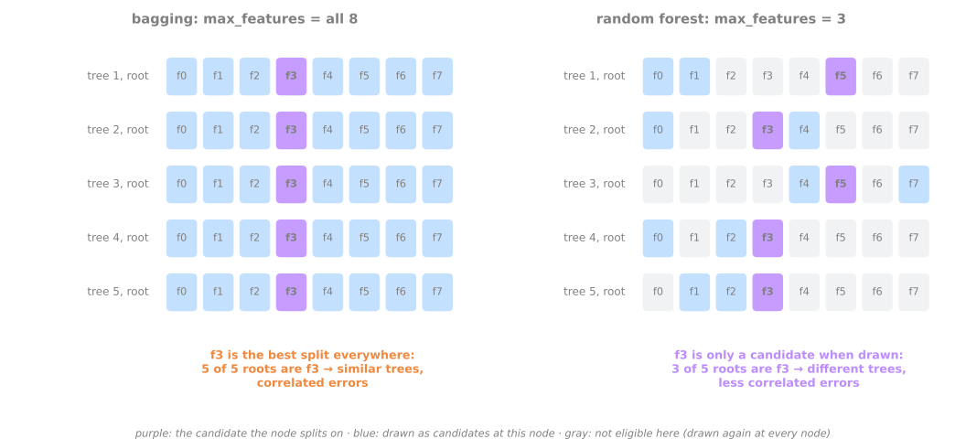
Cada árvore fica mais fraca, já que muitas vezes lhe é negada a melhor divisão. As árvores também ficam menos parecidas. A primeira seção diz qual efeito vence: a variância da floresta é \(\rho\sigma^2 + (1-\rho)\sigma^2/B\), então baixar \(\rho\) pode mais do que compensar um \(\sigma^2\) maior. No conjunto digits (1.797 dígitos manuscritos, 8×8 = 64 pixels cada), com validação cruzada 5-fold numa parte de treino (aula de validação cruzada):
import pandas as pd
from sklearn.datasets import load_digits
from sklearn.ensemble import RandomForestClassifier
from sklearn.model_selection import StratifiedKFold, train_test_split

X, y = load_digits(return_X_y=True)                    # 1.797 imagens de 8×8 pixels, dígitos 0-9
X_train, X_test, y_train, y_test = train_test_split(X, y, test_size=0.25, stratify=y, random_state=0)
cv = StratifiedKFold(n_splits=5, shuffle=True, random_state=0)

rows = []
for m in [64, 20, 8, 3, 1]:                            # 64 = todos os pixels = bagging puro; 8 = sqrt(64)
    corr, tree_err, forest_err, roots = [], [], [], []
    for tr, va in cv.split(X_train, y_train):
        rf = RandomForestClassifier(n_estimators=200, max_features=m, random_state=0, n_jobs=-1)
        rf.fit(X_train[tr], y_train[tr])
        Xv, yv = X_train[va], y_train[va]
        wrong = np.array([rf.classes_[t.predict(Xv).astype(int)] != yv for t in rf.estimators_])
        C = np.corrcoef(wrong)                         # 200 × 200: duas árvores erram nas mesmas linhas?
        corr.append(np.nanmean(C[np.triu_indices(200, 1)]))
        tree_err.append(wrong.mean())
        forest_err.append(1 - rf.score(Xv, yv))
        roots += [t.tree_.feature[0] for t in rf.estimators_]
    top_root = pd.Series(roots).value_counts().iloc[0] / len(roots)
    rows.append({'max_features': m, 'same root pixel': f"{top_root:.0%}",
                 'correlation': round(np.mean(corr), 3), 'one tree error': round(np.mean(tree_err), 3),
                 'forest error': round(np.mean(forest_err), 3)})
print(pd.DataFrame(rows).to_string(index=False))
 max_features same root pixel  correlation  one tree error  forest error
           64             66%        0.304           0.195         0.053
           20             24%        0.233           0.215         0.027
            8             10%        0.198           0.249         0.023
            3              6%        0.160           0.309         0.025
            1              4%        0.133           0.375         0.030
Para cada floresta, wrong registra quais imagens de validação cada árvore erra; correlation é a correlação média entre os erros de duas árvores: 1 significaria que elas sempre falham nas mesmas imagens, 0 que suas falhas não têm relação. Leia a tabela de cima para baixo:
- Bagging puro (todos os 64 pixels): 66% das árvores perguntam sobre o mesmo pixel na raiz. Seus erros têm correlação 0,304. Cada árvore erra 19,5% das imagens; a floresta, 5,3%.
max_features = 8(\(\sqrt{64}\), o padrão do scikit-learn para classificação): só 10% das raízes coincidem e a correlação cai para 0,198. Cada árvore é pior (24,9% de erro), mas a floresta fica mais de duas vezes melhor: 2,3% de erro.max_features = 1: cada divisão pega um pixel ao acaso e só escolhe o limiar. A correlação continua caindo (0,133), mas as árvores agora são tão fracas (37,5% de erro) que a floresta volta a piorar (3,0%).
A figura repete o experimento para doze valores de max_features (script da figura):
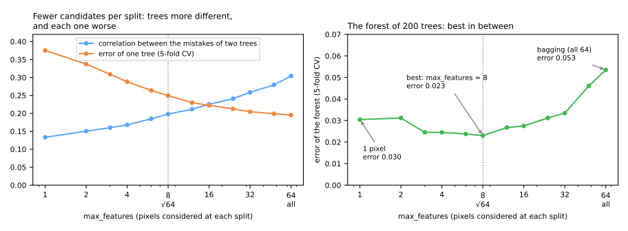
É o compromisso força–correlação de Breiman: a floresta quer árvores fortes e descorrelacionadas; max_features troca uma coisa pela outra. O ótimo costuma ser largo e fica numa pequena fração dos atributos; os padrões são \(\sqrt{d}\) para classificação e, no scikit-learn, todos os atributos para regressão (max_features=1.0, o que faz do RandomForestRegressor um bagging puro, a menos que você mude isso; Breiman sugeria \(d/3\)).
Um pouco de história
Tin Kam Ho (1995, 1998) construiu "florestas de decisão aleatórias" crescendo cada árvore num subconjunto aleatório dos atributos, o método dos subespaços aleatórios. Amit & Geman (1997) aleatorizaram os atributos considerados em cada nó, para reconhecer formas. Breiman tinha introduzido o bagging em 1996; seu artigo de 2001 combinou amostras bootstrap com seleção aleatória de atributos em cada divisão, batizou o resultado de random forests e deu a estimativa de erro out-of-bag e a análise de força e correlação usadas nesta aula. Geurts, Ernst & Wehenkel (2006) levaram a aleatorização adiante com as Extra-Trees (abaixo).
5. Avaliação out-of-bag: validação de graça
Linha a linha
Etapa 4. Cada árvore de uma floresta foi crescida numa amostra bootstrap que deixou de fora cerca de 37% das linhas. Para aquela árvore, essas linhas são out-of-bag (OOB), "fora da sacola": dados não vistos. Então toda linha de treino tem um conjunto de árvores que nunca a viu e que podem votar nela. Eis uma floresta de só 10 árvores nos dígitos e duas imagens de treino:
small = RandomForestClassifier(n_estimators=10, random_state=0).fit(X_train, y_train)
for row in [15, 7]:
    print(f"row {row} (true digit {y_train[row]}):")
    for b, (tree, drawn) in enumerate(zip(small.estimators_, small.estimators_samples_)):
        times = (drawn == row).sum()                   # quantas vezes o bootstrap sorteou esta linha
        if times == 0:
            print(f"   tree {b}: out-of-bag, votes {int(tree.predict(X_train[[row]])[0])}")
row 15 (true digit 7):
   tree 0: out-of-bag, votes 4
   tree 2: out-of-bag, votes 7
   tree 3: out-of-bag, votes 7
   tree 7: out-of-bag, votes 4
   tree 8: out-of-bag, votes 7
   tree 9: out-of-bag, votes 7
row 7 (true digit 9):
   tree 0: out-of-bag, votes 9
   tree 2: out-of-bag, votes 3
   tree 6: out-of-bag, votes 3
   tree 8: out-of-bag, votes 3
A imagem 15 (um 7) ficou de fora de 6 das 10 árvores; quatro delas votam 7 e duas votam 4, então sua previsão OOB é 7, correta. A imagem 7 (um 9) ficou de fora de 4 árvores, três das quais votam 3: sua previsão OOB está errada. Fazer isso para toda linha de treino e contar os erros dá o erro OOB; 1 menos ele é o oob_score_. (O scikit-learn tira a média das probabilidades previstas pelas árvores OOB em vez de contar votos; com árvores completas, cujas folhas são quase sempre puras, as duas coisas coincidem.) Nenhuma linha foi avaliada por uma árvore que treinou nela, então a estimativa é honesta e não custa nenhum ajuste extra.
OOB contra validação cruzada e o conjunto de teste
from sklearn.model_selection import cross_val_score

rf = RandomForestClassifier(n_estimators=500, oob_score=True, random_state=0, n_jobs=-1)
rf.fit(X_train, y_train)
cv_acc = cross_val_score(RandomForestClassifier(n_estimators=500, random_state=0, n_jobs=-1),
                         X_train, y_train, cv=cv)
print(f"OOB accuracy        {rf.oob_score_:.3f}   (1 fit)")
print(f"5-fold CV accuracy  {cv_acc.mean():.3f} ± {cv_acc.std():.3f}   (5 fits)")
print(f"test accuracy       {rf.score(X_test, y_test):.3f}   (450 untouched images)")
OOB accuracy        0.975   (1 fit)
5-fold CV accuracy  0.977 ± 0.007   (5 fits)
test accuracy       0.976   (450 untouched images)
Três estimativas da mesma coisa, que diferem entre si em no máximo 0,002: a estimativa OOB é tão boa quanto a CV 5-fold aqui, a um quinto do custo. Cada previsão OOB vem de uma subfloresta com cerca de 37% das árvores, treinadas em cerca de 63% das linhas distintas, então ela é, se tanto, levemente pessimista, como uma CV com folds de treino pequenos. O OOB é prático para verificações rápidas, para curvas de aprendizado em n_estimators e para escolher um limiar de decisão sem um split de validação separado (o lab faz exatamente isso). Ele não substitui uma validação cruzada de verdade quando você compara uma floresta com outros modelos: eles não têm estimativa OOB; além disso, comparações precisam dos mesmos folds para todos (aula de validação cruzada).
Quantas árvores?
Crescendo uma floresta árvore a árvore (warm_start=True) e registrando o erro OOB, o erro de teste e, em alguns tamanhos, o erro de CV (script da figura):
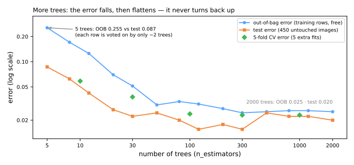
O erro cai rápido, depois se estabiliza e nunca volta a subir: mais árvores não sobreajustam, porque cada árvore nova só deixa a média mais estável (o termo \((1-\rho)\sigma^2/B\) encolhe). A parte plana oscila alguns milésimos (uma das 450 imagens de teste vale 0,0022), mas não mostra tendência. O único preço de mais árvores é tempo e memória. A ponta da esquerda mostra também o único caso em que o OOB engana: com 5 árvores, cada linha fica fora da sacola de só umas 2 delas, então sua "floresta" OOB é minúscula; o erro OOB (0,255) é muito pior que o da verdadeira floresta de 5 árvores no teste (0,087). Leia o erro OOB só quando a floresta já tiver algumas dezenas de árvores.
O sobreajuste numa floresta, quando acontece, vem de árvores individuais profundas demais em dados ruidosos (não do número delas) e é controlado com min_samples_leaf ou max_depth.
6. Resumo: a floresta em cinco linhas
- A média corta variância, até um piso. A variância da média de \(n\) membros é \(\rho\sigma^2 + (1-\rho)\sigma^2/n\): o termo compartilhado, \(\rho\sigma^2\), não cai com \(n\).
- O bootstrap dá a cada árvore uma amostra diferente das mesmas linhas; cerca de 37% delas ficam de fora de cada árvore.
- Bagging cresce árvores profundas (viés baixo, variância alta) em amostras bootstrap e tira a média: o viés fica, a variância cai.
max_featuressorteia os candidatos de cada divisão: árvores individualmente piores, mas menos correlacionadas — e uma floresta melhor.- As linhas out-of-bag avaliam a floresta sem um split de validação; mais árvores nunca pioram o erro, só custam tempo.
| sintoma | o que está acontecendo | o que fazer |
|---|---|---|
| a curva de erro OOB estacionou | a média já removeu a variância que dava para remover | parar de acrescentar árvores |
| estacionou alto demais | viés das árvores ou correlação entre elas | árvores mais fundas, outro max_features, atributos melhores |
| erro OOB muito pior que o de teste | poucas árvores: cada linha tem poucos votos OOB | só ler o OOB com algumas dezenas de árvores |
| a floresta pouco melhor que o bagging | um atributo forte domina todas as raízes | baixar max_features |
Lab fundamental — um filtro de spam com florestas
O problema. O conjunto Spambase (Hopkins et al., 1999) foi coletado no Hewlett-Packard Labs: 4.601 e-mails, cada um descrito por 57 números: a frequência de 48 palavras e 6 caracteres (free, remove, $, !, ...) e três medidas de sequências de letras maiúsculas. A tarefa: marcar o spam. Você o encontrou na aula de árvores de decisão, onde cinquenta árvores crescidas em reamostragens bootstrap votaram melhor que qualquer uma delas. Aqui construímos a floresta direito e perguntamos o que importa para um filtro de spam: um e-mail legítimo mandado para a pasta de spam é pior que um spam que passa, então a precisão na classe spam importa mais que o recall.
O fluxo é o da aula de validação: trancar um conjunto de teste, comparar modelos nos mesmos folds de validação cruzada e tocar no teste uma única vez, no passo 10. Esta parte vai da árvore única à floresta e mede o que a floresta ganha; o ajuste, o limiar e o teste ficam para o lab avançado.
Como fazer este lab em aula (cerca de 40 min, em duplas)
- Abra o notebook do lab no Colab. Não é preciso baixar nem instalar nada: o Colab roda no navegador. Para guardar as suas respostas, salve uma cópia no seu Drive (Arquivo → Salvar uma cópia no Drive) antes de editar. Rode as células em ordem, numa mesma sessão.
- Este lab corresponde aos passos 1 a 7 do notebook. O lab avançado continua no mesmo notebook, a partir do passo 8.
- Cada passo começa com um Preveja: responda com a dupla antes de rodar a célula. Errar a previsão é o que torna o resultado memorável.
- Depois de rodar, compare com a saída e a leitura desta página. Toda saída aqui é exatamente o que o código imprime.
- As Simulações pedem que vocês escrevam um pequeno experimento em Python: mudar uma entrada e observar o que acontece com a saída. Nada de conta à mão. A solução fica recolhida logo abaixo: tente antes de abrir.
- Ritmo sugerido: passos 1 a 3 em 10 min; passos 4 e 5 e a primeira simulação em 15 min; passos 6 e 7 e a segunda simulação em 15 min. O passo 4 leva alguns segundos para rodar.
Passo 1 — carregar e olhar
Preveja. Que palavras você espera ver com muito mais frequência no spam do que no e-mail legítimo? Alguma palavra poderia indicar "legítimo" só por causa de quem coletou os dados?
import numpy as np
import pandas as pd
from sklearn.datasets import fetch_openml

pd.set_option('display.max_columns', 20)
pd.set_option('display.width', 120)
spam = fetch_openml(data_id=44, as_frame=True)       # Spambase (UCI): 4.601 e-mails
X = spam.data                                        # 57 atributos numéricos
y = (spam.target == '1').astype(int)                 # 1 = spam, 0 = legítimo
print(X.shape)
print(y.value_counts())
tokens = ['word_freq_free', 'word_freq_remove', 'char_freq_%24', 'word_freq_george', 'word_freq_hp']
print(X[tokens].gt(0).groupby(y).mean().round(3))    # fração de e-mails que contêm cada token
(4601, 57)
class
0    2788
1    1813
Name: count, dtype: int64
       word_freq_free  word_freq_remove  char_freq_%24  word_freq_george  word_freq_hp
class
0               0.090             0.015          0.104             0.277         0.373
1               0.546             0.421          0.612             0.004         0.028
4.601 e-mails: 1.813 spams (39,4%) e 2.788 legítimos. Todo atributo é uma frequência (a porcentagem das palavras do e-mail que são free, por exemplo) ou uma contagem, todos não negativos e em escalas muito diferentes; árvores não ligam para isso, então não há padronização em lugar nenhum deste lab. A tabela dá a fração de e-mails que contêm cada token ao menos uma vez, por classe. free, remove e $ são marcas clássicas de spam: remove aparece em 42,1% dos spams e em 1,5% dos legítimos. Os outros dois apontam para o lado oposto: george está em 27,7% dos legítimos e 0,4% dos spams, hp em 37,3% e 2,8%. Isso não é uma lei do spam. Os e-mails legítimos vieram das caixas de correio de trabalho e pessoais das pessoas do HP Labs que montaram o conjunto (George Forman entre elas); a documentação avisa que palavras como george indicam "não spam" só para aquela caixa, o que serve para um filtro personalizado e nada mais. Guarde isso para o passo 11. Um alerta: 394 destes e-mails são cópias exatas de outro, que a aula de árvores de decisão descarta como vazamento por linhas duplicadas. Este lab as mantém, como faz a maioria dos estudos com esse conjunto, então seus escores de validação cruzada e de teste saem um pouco otimistas; refazê-lo depois de X.drop_duplicates() é um bom exercício.
Passo 2 — trancar o conjunto de teste
Preveja. Com 921 e-mails no teste, quanto vale um único e-mail em pontos de acurácia?
from sklearn.model_selection import train_test_split

X_train, X_test, y_train, y_test = train_test_split(
    X, y, test_size=0.2, stratify=y, random_state=42)
print(X_train.shape, X_test.shape)
print(f"spam share: train {y_train.mean():.3f} · test {y_test.mean():.3f}")
3.680 e-mails para desenvolvimento e 921 trancados até o passo 10, os dois com 39,4% de spam graças a stratify=y. No teste, um e-mail vale 0,11 ponto de acurácia.
Passo 3 — um baseline e os folds que todos compartilham
Preveja. Se 39,4% dos e-mails são spam, quanto acerta um modelo que chama tudo de legítimo? E qual é a ROC AUC dele?
from sklearn.dummy import DummyClassifier
from sklearn.model_selection import StratifiedKFold, cross_validate

cv = StratifiedKFold(n_splits=5, shuffle=True, random_state=42)
folds = {}                                           # as 5 notas por fold de cada modelo, para o passo 5


def evaluate(name, model):
    r = cross_validate(model, X_train, y_train, cv=cv, scoring=['accuracy', 'roc_auc'])
    folds[name] = r
    print(f"{name:14s} accuracy {r['test_accuracy'].mean():.3f} ± {r['test_accuracy'].std():.3f} · "
          f"ROC AUC {r['test_roc_auc'].mean():.3f} ± {r['test_roc_auc'].std():.3f}")


evaluate('dummy', DummyClassifier(strategy='most_frequent'))
Chamar tudo de legítimo acerta 60,6% das vezes e não ordena nada (ROC AUC 0,5). Toda acurácia deve ser lida contra 0,606. O objeto cv é criado uma vez e reutilizado por todos os modelos e pela busca em grade, então todas as comparações são feitas nos mesmos cinco folds (aula de validação cruzada); folds guarda as cinco notas de cada modelo para a comparação pareada do passo 5.
Passo 4 — uma árvore, bagging, random forest, Extra-Trees
Preveja. Entre uma árvore e os três ensembles, em qual métrica a diferença vai ser maior, acurácia ou ROC AUC? Por quê?
from sklearn.ensemble import ExtraTreesClassifier, RandomForestClassifier
from sklearn.tree import DecisionTreeClassifier

evaluate('one tree', DecisionTreeClassifier(random_state=0))
evaluate('bagging', RandomForestClassifier(n_estimators=200, max_features=None,   # todos os 57 atributos
                                           random_state=0, n_jobs=-1))
evaluate('random forest', RandomForestClassifier(n_estimators=200, random_state=0, n_jobs=-1))
evaluate('extra-trees', ExtraTreesClassifier(n_estimators=200, random_state=0, n_jobs=-1))
one tree       accuracy 0.916 ± 0.008 · ROC AUC 0.913 ± 0.007
bagging        accuracy 0.940 ± 0.006 · ROC AUC 0.978 ± 0.005
random forest  accuracy 0.953 ± 0.006 · ROC AUC 0.986 ± 0.004
extra-trees    accuracy 0.957 ± 0.007 · ROC AUC 0.987 ± 0.004
Como ler:
- Uma árvore: 91,6% de acurácia, mas ROC AUC de só 0,913. Uma árvore completa tem folhas puras, então suas "probabilidades" são 0 ou 1 e ela não consegue ordenar os e-mails sobre os quais está em dúvida; sua AUC é pouco mais que sua acurácia balanceada.
- Bagging:
RandomForestClassifier(max_features=None)é exatamente o bagging de árvores, já que toda divisão pode usar os 57 atributos. Duzentas árvores sobem a acurácia para 94,0% e, sobretudo, a ROC AUC para 0,978: a fração de árvores votando "spam" é uma nota de granulação fina. - Random forest: deixar cada divisão considerar só 7 atributos sorteados (\(\sqrt{57}\), arredondado para baixo) acrescenta mais 1,3 ponto de acurácia (95,3%) e leva a AUC a 0,986. O efeito da descorrelação medido nos dígitos, de novo.
- Extra-Trees: 95,7% e 0,987, essencialmente o mesmo que a floresta.
Os desvios-padrão (0,004–0,008) são pequenos perto das distâncias entre as três primeiras linhas, mas a comparação justa é fold a fold.
Simulação: a floresta é melhor que as próprias árvores? No primeiro fold do cv, ajuste uma floresta de 200 árvores e meça a acurácia de validação de cada árvore sozinha: a média, a melhor e a pior. Compare com o voto da floresta e com uma única árvore crescida em todas as linhas do fold. Alguma árvore da floresta chega ao voto?
Solução
tr, va = next(cv.split(X_train, y_train))                       # o primeiro fold
Xa, ya, Xv, yv = X_train.iloc[tr], y_train.iloc[tr], X_train.iloc[va], y_train.iloc[va]
forest = RandomForestClassifier(n_estimators=200, random_state=0, n_jobs=-1).fit(Xa, ya)
tree_acc = np.array([np.mean(t.predict(Xv.to_numpy()) == yv.to_numpy()) for t in forest.estimators_])
single = DecisionTreeClassifier(random_state=0).fit(Xa, ya).score(Xv, yv)
print(f"one tree on all the rows: {single:.3f}")
print(f"the forest's 200 trees:   mean {tree_acc.mean():.3f} · best {tree_acc.max():.3f} · worst {tree_acc.min():.3f}")
print(f"the forest's vote:        {forest.score(Xv, yv):.3f}")
one tree on all the rows: 0.928
the forest's 200 trees:   mean 0.900 · best 0.935 · worst 0.861
the forest's vote:        0.961
Cada árvore da floresta acerta em média 0,900, pior que a árvore única crescida em todas as linhas do fold (0,928): ela viu só cerca de 63% dos e-mails distintos e, em cada divisão, só 7 dos 57 atributos. Nem a melhor das 200 (0,935) chega perto do voto: 0,961. A floresta é melhor que todas as suas árvores porque elas erram em e-mails diferentes e o voto cancela os erros que não são compartilhados: é a fórmula da seção 1, com \(\sigma^2\) maior e \(\rho\) bem menor.
Passo 5 — diferenças pareadas, fold a fold
Preveja. A floresta está 1,3 ponto de acurácia à frente do bagging, com desvios entre folds de cerca de 0,006. Isso basta para declarar vitória? Que comparação resolve a dúvida?
for a, b in [('random forest', 'one tree'), ('random forest', 'bagging'), ('extra-trees', 'random forest')]:
    for metric in ['accuracy', 'roc_auc']:
        d = folds[a]['test_' + metric] - folds[b]['test_' + metric]
        print(f"{a} - {b:14s} {metric:8s} {d.round(3)}  ->  {d.mean():+.3f} ± {d.std():.3f}")
random forest - one tree       accuracy [0.033 0.034 0.052 0.031 0.035]  ->  +0.037 ± 0.007
random forest - one tree       roc_auc  [0.065 0.07  0.083 0.076 0.071]  ->  +0.073 ± 0.006
random forest - bagging        accuracy [0.018 0.01  0.011 0.007 0.02 ]  ->  +0.013 ± 0.005
random forest - bagging        roc_auc  [0.006 0.006 0.01  0.01  0.009]  ->  +0.008 ± 0.002
extra-trees - random forest  accuracy [ 0.001  0.005  0.005  0.015 -0.007]  ->  +0.004 ± 0.007
extra-trees - random forest  roc_auc  [ 0.001 -0.001  0.003  0.001  0.001]  ->  +0.001 ± 0.001
Cada linha subtrai as notas de dois modelos no mesmo fold:
- a floresta vence a árvore única em todos os folds, por 0,031 a 0,052 de acurácia (+0,037 ± 0,007) e por 0,065 a 0,083 de ROC AUC (+0,073 ± 0,006);
- a floresta vence o bagging em todos os folds também: +0,013 ± 0,005 de acurácia, +0,008 ± 0,002 de AUC. É o que vale o sorteio de atributos nestes dados;
- Extra-Trees contra a floresta: +0,004 ± 0,007 de acurácia, com um fold indo para o outro lado e +0,001 ± 0,001 de AUC. A diferença média não é maior que sua dispersão: pela regra da aula de validação cruzada, um empate.
Com empate, a escolha é feita por outros critérios. Seguimos com a random forest, porque ela é treinada em amostras bootstrap e portanto tem estimativas out-of-bag, que os próximos passos usam. (As Extra-Trees dispensam o bootstrap por padrão.)
Passo 6 — out-of-bag: a mesma estimativa, com um ajuste
Preveja. Cada árvore deixa de fora cerca de 37% dos e-mails. Uma estimativa feita só com as árvores que não viram cada e-mail vai ficar perto da validação cruzada, bem acima ou bem abaixo dela?
from sklearn.metrics import roc_auc_score

rf = RandomForestClassifier(n_estimators=200, oob_score=True, random_state=0, n_jobs=-1)
rf.fit(X_train, y_train)                             # um ajuste, em todo o X_train
p_oob = rf.oob_decision_function_[:, 1]              # cada e-mail avaliado só por árvores que nunca o viram
print(f"OOB: accuracy {rf.oob_score_:.3f} · ROC AUC {roc_auc_score(y_train, p_oob):.3f}   (1 fit)")
print(f"CV:  accuracy {folds['random forest']['test_accuracy'].mean():.3f} · "
      f"ROC AUC {folds['random forest']['test_roc_auc'].mean():.3f}   (5 fits)")
in_bag = np.array([np.isin(np.arange(len(X_train)), s) for s in rf.estimators_samples_])
n_oob = (~in_bag).sum(axis=0)                        # árvores que NÃO viram cada e-mail
print(f"out-of-bag trees per e-mail: mean {n_oob.mean():.1f} of 200 · min {n_oob.min()} · max {n_oob.max()}")
OOB: accuracy 0.953 · ROC AUC 0.986   (1 fit)
CV:  accuracy 0.953 · ROC AUC 0.986   (5 fits)
out-of-bag trees per e-mail: mean 73.6 of 200 · min 47 · max 100
A estimativa OOB reproduz a CV 5-fold até a terceira casa decimal: acurácia 0,953 e ROC AUC 0,986 dos dois jeitos, com um ajuste em vez de cinco. A última linha mostra por que funciona: cada e-mail ficou de fora de 73,6 das 200 árvores em média (36,8%, o \(1/e\) da seção de bootstrap) e nunca de menos de 47. Essas árvores formam uma floresta respeitável que nunca viu o e-mail.
oob_decision_function_ guarda, para cada e-mail de treino, a probabilidade de spam calculada só por essas árvores. É uma nota honesta, fora da amostra, para toda linha de treino, que o passo 9 usa para escolher um limiar.
Passo 7 — quantas árvores?
Preveja. Passadas algumas dezenas de árvores, o erro OOB continua caindo, estaciona ou volta a subir?
import matplotlib.pyplot as plt

growing = RandomForestClassifier(warm_start=True, oob_score=True, random_state=0, n_jobs=-1)
sizes, oob_error = [10, 25, 50, 100, 200, 400], []
for B in sizes:
    growing.set_params(n_estimators=B).fit(X_train, y_train)   # warm_start: só as árvores novas são crescidas
    oob_error.append(1 - growing.oob_score_)
print(pd.Series(oob_error, index=pd.Index(sizes, name='trees'), name='OOB error').round(4).to_string())
plt.plot(sizes, oob_error, 'o-')
plt.xscale('log'); plt.xlabel('number of trees'); plt.ylabel('OOB error')
plt.show()
O erro OOB cai de 7,55% com 10 árvores para 4,62% com 100 e depois fica estável: 4,67% com 200, 4,57% com 400. Um e-mail vale 0,027 ponto de erro OOB, então os três últimos valores diferem por 2 a 4 e-mails: ruído, não tendência. Duzentas árvores bastam para comparar configurações; o modelo final do passo 9 usa 500, o que só custa tempo.
Simulação: árvores rasas, quantas forem. O passo 7 mostrou o erro OOB estacionar com árvores completas. Repita com árvores de profundidade 3 (max_depth=3), para 10, 50, 200 e 400 árvores. Acrescentar árvores leva a floresta rasa até o erro da floresta de árvores completas?
Solução
print('trees   full trees   depth 3')
for B in [10, 50, 200, 400]:
    errs = []
    for depth in [None, 3]:
        f = RandomForestClassifier(n_estimators=B, max_depth=depth, oob_score=True, random_state=0, n_jobs=-1)
        errs.append(1 - f.fit(X_train, y_train).oob_score_)
    print(f"{B:5d}   {errs[0]:10.4f}   {errs[1]:7.4f}")
As duas curvas estacionam, mas em lugares diferentes: a floresta de árvores completas perto de 4,6% de erro OOB e a de árvores rasas perto de 8,7–8,9%, quase o dobro. De 200 para 400 árvores a floresta rasa nem melhora (0,0867 → 0,0886, uma diferença de sete e-mails: ruído). A média remove variância; o erro de uma árvore de profundidade 3 é sobretudo viés — oito folhas não bastam para separar spam de e-mail legítimo — e 400 cópias de um modelo enviesado continuam enviesadas. É por isso que florestas usam árvores profundas.
Para fechar a parte fundamental. Em uma frase cada: (1) por que o voto de 200 árvores acerta mais que a melhor delas? (2) Por que o erro OOB é honesto, se toda árvore foi treinada no X_train? (3) Em que situação acrescentar árvores não ajuda nada?
Sua vez (fundamental)
Para casa:
- Sem as duplicatas. Refaça os passos 3 a 6 depois de
X = X.drop_duplicates()(e doycorrespondente). Quanto caem a acurácia e a ROC AUC de CV? O erro OOB acompanha a queda? - Amostras bootstrap menores. Use
max_samples=0.2(cada árvore vê 20% das linhas) e depois0.5; compare a ROC AUC de CV e o tempo de ajuste com o padrão. Quantas árvores out-of-bag cada e-mail recebe agora? A estimativa OOB continua perto da CV? - Uma prévia da aula de gradient boosting. Acrescente
evaluate('boosting', HistGradientBoostingClassifier(random_state=0))(desklearn.ensemble) ao passo 4 e calcule sua diferença pareada com a random forest em ROC AUC, como no passo 5. É vitória, derrota ou empate?
Abordagem avançada
A parte fundamental construiu a floresta e mostrou por que ela funciona. Esta parte mostra onde a média para de ajudar e como usar a floresta sem se enganar: o voto da maioria sob correlação, quanto do erro do bagging é o piso \(\rho\sigma^2\), quais hiperparâmetros importam de verdade, por que as importâncias da floresta enganam, o que as Extra-Trees mudam e o que uma floresta não consegue fazer. Os blocos de código continuam os das seções 1 a 5.
Esta parte segue um caminho em quatro etapas, desenhado abaixo: 1. por que o voto funciona; 2. ajustar o que importa; 3. ler as importâncias; 4. variantes e limites. Cada etapa leva à sua seção e, nos slides, uma faixa embaixo mostra em que etapa você está.
- Por que o voto funcionao júri de Condorcet; o piso ρσ², medido
- Ajustar o que importa
max_features,min_samples_leaf, árvores suficientes - Ler as importânciasviés da impureza, permutação, crédito dividido
- Variantes e limitesExtra-Trees, sem extrapolação, custo
Slides da abordagem avançada
Clique nos slides e use as setas ← → para navegar; F abre em tela cheia e Esc mostra todos os slides. Abrir os slides numa aba nova
7. Voto da maioria: o teorema do júri de Condorcet
Etapa 1. Classificadores votam em vez de tirar média de números, mas a mesma lógica vale. Em 1785, o Marquês de Condorcet perguntou com que frequência um júri decide corretamente quando cada jurado, independentemente, acerta com probabilidade \(p > 0,5\). Com três jurados e \(p = 0,6\), a maioria acerta quando os três acertam ou exatamente dois acertam:
O fator 3 conta qual dos três jurados é o que erra. Para \(n\) jurados, a probabilidade é uma soma de termos binomiais, um para cada maioria vencedora:
from math import comb


def majority_right(n, p):
    """P(mais da metade de n votantes independentes acerta), cada um acertando com probabilidade p."""
    return sum(comb(n, k) * p**k * (1 - p)**(n - k) for k in range(n // 2 + 1, n + 1))


for n in [1, 3, 11, 101, 1001]:
    print(f"n = {n:4d}: majority right with probability {majority_right(n, 0.6):.4f}")
n =    1: majority right with probability 0.6000
n =    3: majority right with probability 0.6480
n =   11: majority right with probability 0.7535
n =  101: majority right with probability 0.9791
n = 1001: majority right with probability 1.0000
Votantes que acertam só 60% das vezes se tornam, juntos, quase infalíveis: 0,7535 com 11 deles, 0,9791 com 101. A palavra que carrega o teorema inteiro é independentemente. Suponha que cada votante, com probabilidade \(c\), copie uma opinião compartilhada (um jornal que todos leem, um atributo pelo qual toda árvore começa) e, caso contrário, decida sozinho:
def committee(n, p, c, reps=20_000, seed=0):
    """Cada votante copia uma opinião compartilhada com probabilidade c; senão, vota por conta própria."""
    r = np.random.default_rng(seed)
    shared = r.random(reps) < p                  # a opinião compartilhada está certa?
    copies = r.random((reps, n)) < c             # quais votantes a copiam
    own = r.random((reps, n)) < p                # as opiniões independentes
    right = np.where(copies, shared[:, None], own)
    return right, (right.sum(axis=1) > n / 2).mean()


for c in [0.0, 0.1, 0.3]:
    right, _ = committee(2, 0.6, c, reps=200_000)
    corr = np.corrcoef(right[:, 0], right[:, 1])[0, 1]
    acc = [committee(n, 0.6, c)[1] for n in [1, 11, 101, 1001]]
    print(f"c = {c:.1f} · correlation of two voters {corr:.2f} · majority right, n = 1/11/101/1001: "
          + '  '.join(f"{a:.3f}" for a in acc))
c = 0.0 · correlation of two voters -0.00 · majority right, n = 1/11/101/1001: 0.601  0.755  0.980  1.000
c = 0.1 · correlation of two voters 0.01 · majority right, n = 1/11/101/1001: 0.601  0.743  0.917  0.998
c = 0.3 · correlation of two voters 0.09 · majority right, n = 1/11/101/1001: 0.601  0.678  0.618  0.597
Cada votante continua acertando 60% das vezes sozinho. Mas com \(c = 0,3\) a correlação entre dois votantes é de apenas 0,09 (\(c^2\), já que os dois precisam copiar). Isso basta para destruir o efeito: um comitê de 1.001 acerta 59,7% das vezes, nada melhor que um único votante. Cerca de 300 dos 1.001 votantes copiam a opinião compartilhada e os outros 700 se dividem 60/40, então o bloco copiado decide toda votação, certa ou errada. O painel da direita da figura da seção 1 mostra as três curvas. Um pouco de correlação (\(c = 0,1\)) atrasa o ganho; mais que isso o mata.
8. Por que o bagging só cortou a variância pela metade
A tabela da seção 3 mostrou o bagging de 100 árvores completas levando a variância de 0,0883 (uma árvore completa) para 0,0413.
Por que só pela metade, se 100 árvores entraram na média? A fórmula da primeira seção responde. As árvores não são independentes: todas foram crescidas a partir dos mesmos 100 pontos, ruído incluído. Cada amostra bootstrap contém cerca de 63% desses pontos, então duas amostras têm cerca de \(0,63^2 \approx 40\%\) dos pontos em comum. Meça \(\sigma^2\) e \(\rho\) das árvores do bagging, ao longo dos 100 conjuntos de treino:
M = np.array(members)                                  # 100 conjuntos de treino × 10 árvores × 100 pontos
sigma2 = M.var(axis=0).mean()                          # variância de UMA árvore do bagging
Z = (M - M.mean(axis=0)) / M.std(axis=0)               # padroniza ao longo dos conjuntos de treino
rho = np.mean([(Z[:, i] * Z[:, k]).mean() for i in range(10) for k in range(i + 1, 10)])
print(f"one bagged tree: variance {sigma2:.4f} · correlation between two of them {rho:.2f}")
print(f"formula rho·σ² + (1 - rho)·σ²/100 = {rho * sigma2 + (1 - rho) * sigma2 / 100:.4f}")
one bagged tree: variance 0.0937 · correlation between two of them 0.44
formula rho·σ² + (1 - rho)·σ²/100 = 0.0417
Uma árvore do bagging tem variância 0,0937 (um pouco mais que uma árvore completa em todos os dados, já que vê só 63% das linhas distintas); duas delas têm correlação 0,44 no mesmo ponto. A fórmula prevê \(0,44 \times 0,0937 + 0,56 \times 0,0937/100 = 0,0417\) para a média de 100; a variância medida do bagging foi 0,0413. Quase toda a variância que resta é o piso \(\rho\sigma^2\): acrescentar árvores não ajudaria. Para descer mais, as árvores precisam ficar menos correlacionadas: é o que faz o sorteio de atributos da seção 4.
9. Hiperparâmetros que importam e os que quase não importam
Etapa 2. Uma random forest tem muitos botões, mas eles não têm a mesma importância. Para ver quais vale a pena ajustar, mude um de cada vez a partir dos padrões e meça a acurácia de CV 5-fold nos dígitos:
base = dict(n_estimators=200, random_state=0, n_jobs=-1)
study = {'n_estimators': [10, 30, 100, 300],
         'max_features': [1, 'sqrt', 0.5, None],
         'min_samples_leaf': [1, 3, 10, 30],
         'max_depth': [3, 6, 10, None],
         'criterion': ['gini', 'entropy']}
for param, values in study.items():
    scores = [cross_val_score(RandomForestClassifier(**{**base, param: v}), X_train, y_train, cv=cv).mean()
              for v in values]
    print(f"{param:16s}" + '  '.join(f"{str(v):>5s}: {s:.3f}" for v, s in zip(values, scores))
          + f"   range {max(scores) - min(scores):.3f}")
n_estimators       10: 0.941     30: 0.962    100: 0.976    300: 0.977   range 0.036
max_features        1: 0.970   sqrt: 0.977    0.5: 0.967   None: 0.947   range 0.030
min_samples_leaf    1: 0.977      3: 0.972     10: 0.947     30: 0.915   range 0.062
max_depth           3: 0.888      6: 0.957     10: 0.977   None: 0.977   range 0.089
criterion        gini: 0.977  entropy: 0.979   range 0.002
O desvio-padrão entre folds dessas notas é de cerca de 0,007 (medido na seção de OOB), então diferenças abaixo de 0,01 são ruído.
n_estimatorsimporta até a curva achatar (0,941 com 10 árvores, 0,976 com 100) e não depois (0,977 com 300). Escolha "o suficiente", confira a curva OOB e pare.max_featuresé o botão próprio da floresta: o padrãosqrté o melhor (0,977);None(bagging) perde 3 pontos. Em outros dados o ótimo pode mudar, então é a primeira coisa a ajustar.min_samples_leafemax_depthcontrolam a profundidade de cada árvore. Os padrões (árvores completas) são os melhores aqui: florestas querem árvores profundas e de viés baixo, deixando que a média remova a variância. Árvores rasas (profundidade 3: 0,888; folhas de pelo menos 30 imagens: 0,915) acrescentam um viés que nenhuma média remove. Em dados muito ruidosos, ummin_samples_leafmoderado (5–20) pode ajudar e ainda deixa o modelo menor.criterion(Gini ou entropia) não muda nada mensurável (amplitude 0,002), como numa árvore única.class_weight('balanced'ou'balanced_subsample', que recalcula os pesos em cada amostra bootstrap) é para classes desbalanceadas, como oclass_weightda aula de ROC e dados desbalanceados; os dígitos são balanceados, então ele não é estudado aqui.
Na prática: comece dos padrões com algumas centenas de árvores, ajuste max_features e min_samples_leaf com uma pequena busca em grade no seu cv e gaste o esforço que sobrar em atributos. O lab faz exatamente isso. Buscas maiores (busca aleatória, successive halving, otimização bayesiana) são o assunto de AutoML.
10. Importância de atributos
Etapa 3. Uma floresta de centenas de árvores não pode mais ser lida como um fluxograma, então a pergunta "quais atributos ela usa?" precisa ser respondida com um número por atributo. O scikit-learn oferece dois, que podem discordar bastante.
- Importância por impureza (MDI, mean decrease in impurity,
feature_importances_): para cada atributo, some a redução de impureza de toda divisão que o usa, ponderada pela fração de linhas que chegam àquela divisão, tire a média entre as árvores e normalize para somar 1. Ela é calculada nos dados de treino, como subproduto do ajuste, então sai de graça. A aula de árvores de decisão mostrou seu viés numa árvore única. - Importância por permutação (
sklearn.inspection.permutation_importance): em dados separados, embaralhe uma coluna (o que quebra sua ligação com o alvo mas mantém sua distribuição) e meça quanto a nota cai. Repita algumas vezes e tire a média. Custa uma passada de previsão por coluna e repetição; funciona para qualquer modelo. Ela é aprofundada em Explicabilidade.
Muitos valores distintos atraem divisões
Strobl et al. (2007) mostraram que a MDI favorece atributos com muitos pontos de corte possíveis. Para medir isso, tome os dados de crédito alemão (1.000 empréstimos, 20 atributos, 30% de maus pagadores) e acrescente duas colunas de puro ruído: um número de série com 1.000 valores distintos e um cara-ou-coroa com 2:
from sklearn.datasets import fetch_openml
from sklearn.inspection import permutation_importance

credit = fetch_openml(data_id=31, as_frame=True)       # crédito alemão: 1.000 empréstimos, 20 atributos
Xc = credit.data.copy()
for col in Xc.select_dtypes('category'):
    Xc[col] = Xc[col].cat.codes                        # categorias -> códigos inteiros (ok para árvores)
yc = (credit.target == 'bad').astype(int)              # 1 = mau pagador (30%)
rng = np.random.default_rng(0)
Xc['random_id'] = rng.permutation(len(Xc))             # um número de série: 1.000 valores distintos, sem sinal
Xc['coin'] = rng.integers(0, 2, len(Xc))               # um cara-ou-coroa: 2 valores, sem sinal
Xc_tr, Xc_te, yc_tr, yc_te = train_test_split(Xc, yc, test_size=0.3, stratify=yc, random_state=0)

forest = RandomForestClassifier(n_estimators=300, random_state=0, n_jobs=-1).fit(Xc_tr, yc_tr)
perm = permutation_importance(forest, Xc_te, yc_te, scoring='roc_auc', n_repeats=10,
                              random_state=0, n_jobs=-1)
imp = pd.DataFrame({'distinct values': Xc.nunique(),
                    'MDI': forest.feature_importances_,
                    'permutation': perm.importances_mean,
                    '± std': perm.importances_std})
imp['MDI rank'] = imp['MDI'].rank(ascending=False).astype(int)
imp['perm rank'] = imp['permutation'].rank(ascending=False).astype(int)
print(imp.sort_values('MDI', ascending=False).head(6).round(3).to_string())
print(imp.loc[['coin']].round(3).to_string())
                 distinct values    MDI  permutation  ± std  MDI rank  perm rank
credit_amount                921  0.129        0.007  0.013         1          8
random_id                   1000  0.099        0.002  0.007         2         14
duration                      33  0.087        0.056  0.014         3          2
age                           53  0.087        0.013  0.010         4          4
checking_status                4  0.086        0.144  0.026         5          1
purpose                       10  0.060        0.003  0.006         6         10
      distinct values   MDI  permutation  ± std  MDI rank  perm rank
coin                2  0.02       -0.002  0.003        17         22
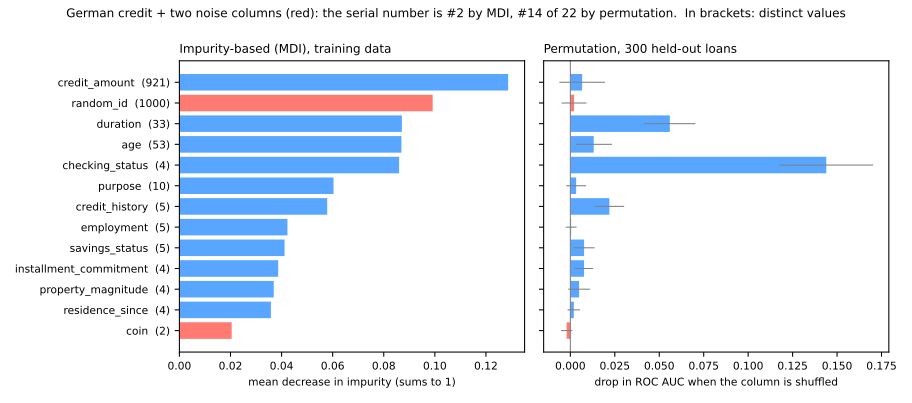
O número de série, ruído por construção, é o segundo atributo mais importante pela MDI (0,099), à frente da duração do empréstimo, da idade do cliente e da situação da conta corrente. A importância por permutação nos 300 empréstimos separados o coloca em 14º de 22, com uma queda de ROC AUC de 0,002 ± 0,007, menor que o próprio desvio-padrão: embaralhá-lo não muda nada, como deveria. O cara-ou-coroa, com só 2 valores, é o 17º pela MDI e o último (22º) pela permutação: poucos valores distintos, poucas chances de ajustar ruído.
O mecanismo é o da aula de árvores de decisão, multiplicado por 300 árvores. No fundo de cada árvore, os nós têm um punhado de linhas, enquanto uma coluna com 1.000 valores distintos oferece centenas de limiares; um deles sempre separa essas poucas linhas um pouco melhor por acaso. Assim, o número de série é escolhido repetidas vezes e cada divisão dessas soma na sua MDI. Essa redução de impureza é medida nas linhas de treino, onde o ruído ajustado de fato "reduz a impureza". O mesmo viés infla atributos reais com muitos valores: credit_amount (921 valores distintos) é o primeiro pela MDI, mas só o 8º pela permutação, enquanto checking_status (4 valores) é o 5º pela MDI e o primeiro pela permutação, com folga (script da figura):
Atributos correlacionados dividem o crédito
A importância por permutação tem um ponto cego próprio. Ela pergunta "quanto pior fica o modelo se esta coluna sozinha for embaralhada?". Se outra coluna carrega a mesma informação, a resposta é "não muito". O teste mais limpo é uma duplicata exata:
def importances(X_tr, X_te, cols):
    f = RandomForestClassifier(n_estimators=300, random_state=0, n_jobs=-1).fit(X_tr, yc_tr)
    p = permutation_importance(f, X_te, yc_te, scoring='roc_auc', n_repeats=10, random_state=0, n_jobs=-1)
    i = [list(X_tr.columns).index(c) for c in cols]
    return pd.DataFrame({'MDI': f.feature_importances_[i], 'permutation': p.importances_mean[i]}, index=cols)


print(importances(Xc_tr, Xc_te, ['checking_status']).round(3))
twin_tr = Xc_tr.assign(checking_copy=Xc_tr['checking_status'])   # uma coluna duplicada, idêntica
twin_te = Xc_te.assign(checking_copy=Xc_te['checking_status'])
print(importances(twin_tr, twin_te, ['checking_status', 'checking_copy']).round(3))
                   MDI  permutation
checking_status  0.086        0.144
                   MDI  permutation
checking_status  0.057        0.049
checking_copy    0.059        0.054
A informação é a mesma, mas com uma gêmea na tabela as duas cópias dividem a MDI (0,086 vira 0,057 + 0,059) e a importância por permutação de cada uma cai para cerca de um terço (0,144 vira 0,049 e 0,054). O que faz as árvores usarem as duas gêmeas é o próprio max_features: em muitos nós só uma das duas é sorteada como candidata, então a floresta aprende a usar qualquer uma delas; embaralhar uma deixa a outra fazer o trabalho. Dados reais estão cheios de quase-gêmeas (raio, perímetro e área do mesmo tumor; renda e imposto pago); um atributo que parece sem importância pode simplesmente ter um substituto. Duas regras práticas decorrem daí:
- prefira a importância por permutação em dados separados à MDI, sobretudo quando os atributos diferem no número de valores distintos;
- antes de concluir que um atributo não importa, confira seus parceiros correlacionados: permute ou retire o grupo inteiro de uma vez ou examine o modelo com ferramentas que levam em conta interações, como o SHAP, em Explicabilidade.
11. Extra-Trees e florestas de regressão
Extra-Trees: limiares aleatórios também
Etapa 4. As árvores extremamente aleatorizadas (Geurts, Ernst & Wehenkel, 2006) vão um passo além: em cada nó, para cada um dos max_features atributos candidatos, sorteiam um limiar aleatório em vez de procurar o melhor e ficam com a melhor dessas divisões aleatórias. Por padrão, também dispensam o bootstrap e crescem cada árvore em todas as linhas. As árvores ficam ainda menos correlacionadas e cada divisão sai mais barata, já que não há busca de limiar. Muda um import:
from sklearn.ensemble import ExtraTreesClassifier

for name, model in [('random forest', RandomForestClassifier(n_estimators=300, random_state=0, n_jobs=-1)),
                    ('extra-trees', ExtraTreesClassifier(n_estimators=300, random_state=0, n_jobs=-1))]:
    s = cross_val_score(model, X_train, y_train, cv=cv)
    nodes = np.mean([t.tree_.node_count for t in model.fit(X_train, y_train).estimators_])
    print(f"{name:14s} CV accuracy {s.mean():.3f} ± {s.std():.3f} · {nodes:.0f} nodes per tree")
random forest  CV accuracy 0.977 ± 0.010 · 329 nodes per tree
extra-trees    CV accuracy 0.981 ± 0.007 · 687 nodes per tree
Nos dígitos, as Extra-Trees ficam ligeiramente à frente (0,981 contra 0,977, bem dentro de um desvio-padrão). Suas árvores têm o dobro de nós (687 contra 329), já que limiares aleatórios dividem com menos eficiência, o que custa memória e tempo de previsão. É uma candidata que merece uma linha em qualquer comparação, como no lab.
Florestas de regressão e o que elas não conseguem fazer
O RandomForestRegressor tira a média de árvores de regressão exatamente como o classificador junta votos. Ele herda uma limitação das suas árvores (aula de árvores de decisão): toda previsão é uma média de alvos de treino, então ele não consegue prever fora da faixa de alvos que já viu. Treine numa reta \(y = 3x\) para \(0 \le x \le 10\) e pergunte sobre \(x\) maiores:
from sklearn.ensemble import RandomForestRegressor
from sklearn.linear_model import LinearRegression

rng = np.random.default_rng(1)
x = np.linspace(0, 10, 100).reshape(-1, 1)              # os dados de treino só cobrem 0 <= x <= 10
y_line = 3 * x[:, 0] + rng.normal(0, 1, 100)           # uma reta, y = 3x, mais ruído
x_new = np.array([[5], [10], [12], [20]])
print("x =            ", x_new[:, 0])
print("truth 3x:      ", 3 * x_new[:, 0])
print("random forest: ", RandomForestRegressor(random_state=0).fit(x, y_line).predict(x_new).round(1))
print("linear model:  ", LinearRegression().fit(x, y_line).predict(x_new).round(1))
x =             [ 5 10 12 20]
truth 3x:       [15 30 36 60]
random forest:  [15.6 29.6 29.6 29.6]
linear model:   [14.9 29.8 35.8 59.7]
Dentro da faixa de treino, a floresta vai bem (15,6 para 15). Fora dela, prevê 29,6 em \(x = 12\) e em \(x = 20\): a média das últimas folhas, uma linha reta horizontal, por mais longe que você vá. O modelo linear extrapola a tendência (59,7 para 60). Para alvos que crescem com o tempo (vendas, preços), modele a tendência separadamente ou preveja variações em vez de níveis.
12. Perfil prático
Uma floresta são as árvores da aula de árvores de decisão, multiplicadas. Isso tem um custo em tamanho, fácil de contar:
import pickle
from sklearn.tree import DecisionTreeClassifier

models = {'one tree': DecisionTreeClassifier(random_state=0),
          'forest': RandomForestClassifier(n_estimators=300, random_state=0, n_jobs=-1),
          'forest, leaf 3': RandomForestClassifier(n_estimators=300, min_samples_leaf=3,
                                                   random_state=0, n_jobs=-1)}
for name, model in models.items():
    acc = cross_val_score(model, X_train, y_train, cv=cv).mean()
    model.fit(X_train, y_train)
    trees = getattr(model, 'estimators_', [model])        # as árvores de uma floresta ou a própria árvore
    print(f"{name:14s} CV accuracy {acc:.3f} · {len(trees):3d} tree(s) · "
          f"{sum(t.tree_.node_count for t in trees):6d} nodes · "
          f"depth {np.mean([t.get_depth() for t in trees]):4.1f} · {len(pickle.dumps(model)) / 1e6:5.2f} MB")
one tree       CV accuracy 0.829 ·   1 tree(s) ·    293 nodes · depth 14.0 ·  0.04 MB
forest         CV accuracy 0.977 · 300 tree(s) ·  98696 nodes · depth 13.2 · 14.32 MB
forest, leaf 3 CV accuracy 0.971 · 300 tree(s) ·  65754 nodes · depth 11.7 ·  9.57 MB
Nos dígitos, uma árvore acerta 0,829 e a floresta 0,977, mas a floresta guarda mais de 300 vezes mais nós: 14,32 MB depois de salva, para um conjunto de treino de 1.347 imagens pequenas, contra 0,04 MB da árvore. Cada previsão percorre 300 caminhos da raiz à folha, de profundidade em torno de 13, em vez de um. Ainda é rápido: as árvores são independentes, então a previsão se paraleliza entre núcleos. Mas árvores completas têm mais ou menos uma folha para cada punhado de linhas de treino, então o tamanho cresce com os dados, o que pesa num celular ou atrás de uma API de baixa latência. Folhas maiores encolhem o modelo: min_samples_leaf=3 economiza um terço da memória (9,57 MB) por 0,006 de acurácia.
| Uma árvore de decisão | Random forest | Gradient boosting | |
|---|---|---|---|
| Árvores | uma, podada | centenas, profundas, independentes | centenas, rasas, sequenciais |
| Ataca | — | variância (média) | viés (cada árvore corrige os erros anteriores) |
| Ajuste necessário | profundidade / poda | pouco: max_features, tamanho da folha | mais: taxa de aprendizado, número de árvores, profundidade |
| Treino | rápido | paralelo entre árvores | sequencial (existem bibliotecas rápidas) |
| Estimativa de validação | CV | OOB de graça ou CV | CV / early stopping |
| Legível | sim, um fluxograma | não; importâncias | não; importâncias |
| Extrapola | não | não | não |
| Quando usar | o modelo precisa ser lido ou auditado | um baseline forte e robusto com pouco esforço | os últimos pontos de acurácia em dados tabulares |
Os pontos fortes da floresta: acurácia excelente com os padrões; robusta a outliers e a transformações monótonas dos atributos, já que as divisões só comparam valores; dispensa padronização; captura interações; estimativa OOB; treino paralelo; difícil de usar errado. Os pontos fracos: um modelo grande e lento de consultar, comparado com uma árvore ou um modelo linear; nenhuma estrutura legível; nenhuma extrapolação; e, na maioria dos benchmarks tabulares, um gradient boosting bem ajustado (tema da próxima aula) fica ligeiramente à frente.
Bagging vs boosting
O bagging constrói as árvores de forma independente, em paralelo, para depois tirar a média e cortar a variância. O boosting, tema da próxima aula, as constrói em sequência, cada uma corrigindo os erros das anteriores, o que ataca o viés. Mesmo bloco de construção, estratégias opostas.
Lab avançado — ajustar, escolher o limiar e testar
O lab fundamental terminou com uma floresta padrão de 200 árvores que acerta 95,3% e cuja estimativa OOB reproduz a validação cruzada. Esta parte ajusta os dois botões que importam, usa as probabilidades out-of-bag para escolher um limiar que protege o e-mail legítimo, abre o teste uma vez e pergunta para onde a floresta olha. Continue no mesmo notebook, na mesma sessão: os passos abaixo usam X_train, y_train, cv, folds e roc_auc_score dos passos 1 a 7.
Como fazer este lab em aula (cerca de 30 min, em duplas)
- Continue no notebook do Colab, a partir do passo 8. Se a sessão caiu, rode antes as células dos passos 1 a 7 (Ambiente de execução → Executar anteriores).
- Como no lab fundamental: Preveja antes de rodar, compare com esta página e tente as Simulações antes de abrir a solução.
- Ritmo sugerido: passo 8 e a primeira simulação em 10 min (a grade leva alguns segundos); passos 9 e 10 em 10 min; passo 11 e a segunda simulação em 10 min.
Passo 8 — ajustar max_features e min_samples_leaf
Preveja. Menos atributos por divisão deixam cada árvore mais fraca. Você espera o melhor max_features perto de 1, perto do padrão (7) ou perto de 57? E folhas de 1 ou de 5 e-mails?
from sklearn.model_selection import GridSearchCV

grid = GridSearchCV(RandomForestClassifier(n_estimators=200, random_state=0, n_jobs=-1),
                    {'max_features': [1, 2, 4, 7, 15], 'min_samples_leaf': [1, 5]},
                    cv=cv, scoring='roc_auc')
grid.fit(X_train, y_train)
res = pd.DataFrame(grid.cv_results_)
print(res.pivot(index='param_min_samples_leaf', columns='param_max_features',
                values='mean_test_score').round(4))
best_std = res.loc[grid.best_index_, 'std_test_score']
print(f"best: {grid.best_params_} · ROC AUC {grid.best_score_:.4f} ± {best_std:.4f}")
ties = res[res['mean_test_score'] >= grid.best_score_ - best_std]
print(f"{len(ties)} of {len(res)} configurations within one std of the best:",
      list(zip(ties['param_max_features'], ties['param_min_samples_leaf'])))
param_max_features          1       2       4       7       15
param_min_samples_leaf
1                       0.9881  0.9875  0.9871  0.9857  0.9835
5                       0.9771  0.9804  0.9818  0.9823  0.9804
best: {'max_features': 1, 'min_samples_leaf': 1} · ROC AUC 0.9881 ± 0.0029
4 of 10 configurations within one std of the best: [(1, 1), (2, 1), (4, 1), (7, 1)]
Dois padrões:
- Folhas de 1 vencem folhas de 5 para todo valor de
max_features, menos um: a floresta quer árvores profundas, como nos dígitos. - Menos atributos por divisão é melhor, devagar: de 0,9835 com 15 atributos para 0,9881 com 1. Com
max_features=1, cada divisão pega um atributo ao acaso e só escolhe o limiar: nestes dados, a descorrelação máxima compensa.
O vencedor é max_features=1, min_samples_leaf=1, com ROC AUC 0,9881 ± 0,0029. Mas quatro das dez configurações estão a menos de um desvio-padrão dele, incluindo o padrão (max_features=7, 0,9857). O ajuste rendeu 0,0024 de AUC, menos que o ruído de um fold para outro: os padrões da floresta são difíceis de bater. Ficamos com o vencedor da grade, que também é o mais rápido de treinar, já que cada divisão examina um único atributo. Seu 0,9881 é a melhor de dez notas medidas nos folds que o escolheram, então é levemente otimista (a maldição do vencedor da aula de validação cruzada).
Simulação: a busca de graça, com o OOB. A grade do passo 8 fez 50 ajustes (10 configurações × 5 folds). Refaça a linha de min_samples_leaf=1 com um único ajuste por configuração, lendo a ROC AUC das probabilidades out-of-bag (oob_decision_function_). O OOB ordena os valores de max_features como a validação cruzada?
Solução
print('max_features   OOB ROC AUC   CV ROC AUC (grid)')
cv_auc = res[res['param_min_samples_leaf'] == 1].set_index('param_max_features')['mean_test_score']
for m in [1, 2, 4, 7, 15]:
    f = RandomForestClassifier(n_estimators=200, max_features=m, oob_score=True, random_state=0, n_jobs=-1)
    f.fit(X_train, y_train)                                    # um ajuste por configuração
    print(f"{m:12d}   {roc_auc_score(y_train, f.oob_decision_function_[:, 1]):11.4f}   {cv_auc[m]:.4f}")
max_features   OOB ROC AUC   CV ROC AUC (grid)
           1        0.9881   0.9881
           2        0.9886   0.9875
           4        0.9873   0.9871
           7        0.9855   0.9857
          15        0.9842   0.9835
Com 5 ajustes em vez de 25, o OOB reproduz a curva da validação cruzada: as duas colunas caem de 1 para 15 atributos e nunca diferem em mais de 0,0011. A ordem dos dois primeiros se inverte (o OOB prefere 2, a CV prefere 1), mas cada coluna os separa por 0,0005–0,0006, bem dentro do desvio entre folds do vencedor (0,0029): é o mesmo empate visto de dois lados. Para uma floresta, o OOB é uma forma barata de varrer um botão; para comparar com modelos de outras famílias, que não têm OOB, continue usando o mesmo cv.
Passo 9 — um limiar que protege o e-mail legítimo, escolhido out-of-bag
Preveja. Para mandar no máximo 1% dos e-mails legítimos para a pasta de spam, o limiar precisa subir ou descer em relação a 0,5? Onde dá para escolhê-lo sem tocar no teste?
final = RandomForestClassifier(n_estimators=500, oob_score=True, random_state=0, n_jobs=-1,
                               **grid.best_params_).fit(X_train, y_train)
p_oob = final.oob_decision_function_[:, 1]
legit = (y_train == 0).to_numpy()
print(" threshold  legit flagged (of 2230)  spam caught")
for t in [0.5, 0.6, 0.65, 0.7, 0.8]:
    flag = p_oob >= t
    print(f"{t:10.2f}  {flag[legit].sum():5d} ({flag[legit].mean():.2%})        {flag[~legit].mean():.1%}")
thresholds = np.arange(0.50, 0.96, 0.05)
chosen = next(t for t in thresholds if (p_oob[legit] >= t).mean() <= 0.01)
print(f"chosen threshold: {chosen:.2f}")
 threshold  legit flagged (of 2230)  spam caught
      0.50     52 (2.33%)        93.2%
      0.60     31 (1.39%)        88.8%
      0.65     25 (1.12%)        86.1%
      0.70     19 (0.85%)        82.8%
      0.80      9 (0.40%)        73.5%
chosen threshold: 0.70
A política vem do problema, não dos dados: no máximo 1% dos e-mails legítimos pode ir para a pasta de spam. Escolher um limiar exige previsões em linhas nas quais o modelo não treinou; na aula de ROC e dados desbalanceados isso custou um split de validação. Aqui as probabilidades out-of-bag as fornecem para todos os 3.680 e-mails de treino, sem custo.
No limiar padrão de 0,5, a floresta marcaria 52 dos 2.230 e-mails legítimos de treino (2,33%), mais que o dobro do orçamento. O primeiro limiar da grade que o respeita é 0,70: 19 e-mails legítimos marcados (0,85%), ainda pegando 82,8% do spam. O limiar agora está fixado, antes de o teste ser aberto.
Passo 10 — o único teste
Preveja. No limiar escolhido, a fração de e-mails legítimos perdidos no teste vai ficar perto dos 0,85% previstos pelo OOB? E o recall de spam, sobe ou cai em relação ao limiar 0,5?
from sklearn.metrics import confusion_matrix, precision_score, recall_score

p_test = final.predict_proba(X_test)[:, 1]
print(f"test ROC AUC {roc_auc_score(y_test, p_test):.3f}")
for t in [0.5, chosen]:
    pred = (p_test >= t).astype(int)
    tp, fn, fp, tn = confusion_matrix(y_test, pred, labels=[1, 0]).ravel()
    print(f"threshold {t:.2f}: legit lost {fp} of {tn + fp} · spam missed {fn} of {fn + tp} · "
          f"precision {precision_score(y_test, pred):.3f} · recall {recall_score(y_test, pred):.3f}")
test ROC AUC 0.984
threshold 0.50: legit lost 14 of 558 · spam missed 32 of 363 · precision 0.959 · recall 0.912
threshold 0.70: legit lost 5 of 558 · spam missed 72 of 363 · precision 0.983 · recall 0.802
A ROC AUC nos 921 e-mails de teste é 0,984, perto da estimativa de CV de 0,988 (que, por ser a melhor de dez configurações, era levemente otimista). Depois, os dois limiares, ambos fixados antes deste passo:
- em 0,5, 14 dos 558 e-mails legítimos vão para o spam (2,5%): precisão 0,959, recall 0,912;
- em 0,70, só 5 vão (0,9%, onde a estimativa OOB tinha previsto 0,85%): precisão 0,983. O preço é o recall: 72 dos 363 spams agora chegam à caixa de entrada, contra 32.
Nove e-mails perdidos a menos custam quarenta spams a mais na caixa de entrada. Se essa troca é a certa, é uma decisão de produto; o que o lab mostra é que ela pode ser feita com previsões out-of-bag e depois confirmada, uma vez, no teste. Relatar as duas linhas não é escolher no teste: nenhum dos limiares foi mudado depois de vê-lo.
Passo 11 — para onde a floresta olha?
Preveja. Uma coluna de números de série, sem nenhum sinal, vai aparecer bem colocada em alguma das duas importâncias? Em qual?
from sklearn.inspection import permutation_importance

rng = np.random.default_rng(0)
Xn_train = X_train.assign(random_id=rng.permutation(len(X_train)))   # mais uma coluna de puro ruído
Xn_test = X_test.assign(random_id=rng.permutation(len(X_test)))
probe = RandomForestClassifier(n_estimators=200, random_state=0, n_jobs=-1,
                               **grid.best_params_).fit(Xn_train, y_train)
perm = permutation_importance(probe, Xn_test, y_test, scoring='roc_auc', n_repeats=10,
                              random_state=0, n_jobs=-1)
imp = pd.DataFrame({'MDI': probe.feature_importances_, 'permutation': perm.importances_mean,
                    '± std': perm.importances_std}, index=Xn_train.columns)
imp['MDI rank'] = imp['MDI'].rank(ascending=False).astype(int)
imp['perm rank'] = imp['permutation'].rank(ascending=False).astype(int)
print(imp.sort_values('permutation', ascending=False).head(10).round(4))
print(imp.loc[['random_id']].round(4))
                     MDI  permutation   ± std  MDI rank  perm rank
char_freq_%21     0.0625       0.0046  0.0013         1          1
word_freq_free    0.0443       0.0039  0.0012         7          2
word_freq_hp      0.0273       0.0037  0.0008        11          3
word_freq_remove  0.0437       0.0033  0.0015         8          4
word_freq_edu     0.0177       0.0030  0.0006        21          5
word_freq_george  0.0162       0.0029  0.0008        25          6
word_freq_you     0.0350       0.0021  0.0006         9          7
word_freq_1999    0.0161       0.0019  0.0003        27          8
word_freq_hpl     0.0177       0.0014  0.0004        20          9
word_freq_re      0.0140       0.0014  0.0004        28         10
              MDI  permutation   ± std  MDI rank  perm rank
random_id  0.0219      -0.0002  0.0004        13         54
Reajustamos a configuração escolhida com uma coluna extra de puro ruído (um número de série aleatório) e comparamos as duas importâncias. A importância por permutação é medida no conjunto de teste: ele já deu seu veredito no passo 10; explicar o modelo não muda nenhuma decisão sobre ele.
Como ler:
- O número de série é o 13º de 58 pela MDI (à frente de 45 atributos reais) e o 54º pela permutação, com uma queda de −0,0002 ± 0,0004: nada. É o viés da árvore única da aula de árvores de decisão (e do exemplo do crédito alemão, acima), agora numa floresta.
- Os dois rankings discordam também nos atributos reais:
georgeé o 25º pela MDI e o 6º pela permutação,1999o 27º e o 8º. Confie na coluna da permutação. - As quedas são pequenas (no máximo 0,0046 de AUC, para
!) porque as palavras se substituem umas às outras: com uma delas embaralhada, as demais ainda identificam a maior parte do spam. - Cinco das dez primeiras (
hp,edu,george,1999,hpl) são rastros de onde vieram os e-mails legítimos: um laboratório de pesquisa, seu pessoal, seus correspondentes. Elas ajudam neste teste (que vem das mesmas caixas de correio), mas enganariam na caixa de qualquer outra pessoa. A importância diz o que o modelo usa, não o que é verdade sobre spam. Uma lista como esta é a melhor forma de pegar um artefato do conjunto de dados antes que ele chegue à produção.
Simulação: a importância de um par de gêmeas. word_freq_857 e word_freq_415 quase sempre aparecem juntas nestes e-mails. No probe do passo 11, meça a queda de ROC AUC no teste ao embaralhar cada uma sozinha e as duas juntas (com a mesma permutação de linhas), dez vezes cada. A queda conjunta é maior que a soma das individuais?
Solução
print(f"correlation: {X_train['word_freq_857'].corr(X_train['word_freq_415']):.3f}")
base_auc = roc_auc_score(y_test, probe.predict_proba(Xn_test)[:, 1])
r2 = np.random.default_rng(0)
drops = {}
for cols in [['word_freq_857'], ['word_freq_415'], ['word_freq_857', 'word_freq_415']]:
    d = []
    for _ in range(10):
        Xs = Xn_test.copy()
        order = r2.permutation(len(Xs))
        Xs[cols] = Xs[cols].to_numpy()[order]                  # a mesma permutação para as colunas juntas
        d.append(base_auc - roc_auc_score(y_test, probe.predict_proba(Xs)[:, 1]))
    drops[' + '.join(cols)] = np.mean(d)
for k, v in drops.items():
    print(f"shuffle {k:30s}: ROC AUC drop {v:.5f}")
correlation: 0.998
shuffle word_freq_857                 : ROC AUC drop 0.00021
shuffle word_freq_415                 : ROC AUC drop 0.00019
shuffle word_freq_857 + word_freq_415 : ROC AUC drop 0.00067
As duas colunas têm correlação 0,998: são quase a mesma informação. Embaralhada sozinha, cada uma quase não faz falta (0,00021 e 0,00019), porque a gêmea cobre. Embaralhadas juntas, a queda é 0,00067, cerca de 1,7 vez a soma das individuais (0,00040). Lida coluna a coluna, a importância por permutação subestima um grupo de atributos correlacionados; é o experimento da gêmea exata da seção 10, agora com dados reais. Os números são pequenos porque estas duas palavras pesam pouco no modelo; a desproporção é o que importa.
Para fechar a aula. Em uma frase cada: (1) por que o vencedor da grade do passo 8 não é melhor que os padrões de forma convincente? (2) Por que as probabilidades out-of-bag servem para escolher o limiar sem gastar o teste? (3) Por que george e hp são importantes neste modelo e inúteis num filtro para outra pessoa?
Sua vez (avançado)
Para casa, com mais tempo:
- Pesos de classe contra limiares. Acrescente
'class_weight': [None, 'balanced_subsample']à grade do passo 8. A ROC AUC do vencedor muda? Reajuste-o com cada opção e compare o limiar OOB que o passo 9 escolhe. Por que pesos de classe e limiares podem acabar fazendo o mesmo trabalho (aula de ROC e dados desbalanceados)? - Sem os rastros do HP Labs. Retire de
Xas colunasword_freq_hp,word_freq_hpl,word_freq_george,word_freq_labs,word_freq_labeword_freq_650e refaça os passos 8 a 10. Quanto a ROC AUC de teste cai? Esse modelo é pior ou só mais honesto? min_samples_leafpelo OOB. Commax_featuresdo vencedor, varramin_samples_leafem 1, 2, 5, 10 e 20 lendo só a ROC AUC out-of-bag, como na simulação do passo 8. Onde está o melhor valor e o que acontece com o tamanho do modelo (sum(t.tree_.node_count for t in f.estimators_))?
Referências
- Galton, F. "Vox Populi." Nature 75 (1907): 450–451 — o concurso de adivinhar o peso do boi. DOI
- Condorcet, Marquês de. Essai sur l'application de l'analyse à la probabilité des décisions rendues à la pluralité des voix. Paris: Imprimerie Royale (1785) — o teorema do júri.
- Efron, B. "Bootstrap Methods: Another Look at the Jackknife." The Annals of Statistics 7, no. 1 (1979): 1–26. DOI
- Breiman, L. "Bagging Predictors." Machine Learning 24, no. 2 (1996): 123–140. DOI
- Ho, T. K. "Random Decision Forests." Proceedings of the 3rd International Conference on Document Analysis and Recognition (ICDAR) (1995): 278–282. DOI
- Amit, Y.; Geman, D. "Shape Quantization and Recognition with Randomized Trees." Neural Computation 9, no. 7 (1997): 1545–1588. DOI
- Ho, T. K. "The Random Subspace Method for Constructing Decision Forests." IEEE Transactions on Pattern Analysis and Machine Intelligence 20, no. 8 (1998): 832–844. DOI
- Breiman, L. "Random Forests." Machine Learning 45, no. 1 (2001): 5–32 — bootstrap mais atributos aleatórios, estimativas out-of-bag, força e correlação. DOI
- Geurts, P.; Ernst, D.; Wehenkel, L. "Extremely Randomized Trees." Machine Learning 63, no. 1 (2006): 3–42. DOI
- Strobl, C.; Boulesteix, A.-L.; Zeileis, A.; Hothorn, T. "Bias in Random Forest Variable Importance Measures: Illustrations, Sources and a Solution." BMC Bioinformatics 8 (2007): 25. DOI
- Hastie, T.; Tibshirani, R.; Friedman, J. The Elements of Statistical Learning, 2ª ed. Springer (2009), capítulo 15 — a variância da média de árvores correlacionadas. DOI
- Hopkins, M.; Reeber, E.; Forman, G.; Suermondt, J. "Spambase." UCI Machine Learning Repository (1999) — o conjunto de dados do lab (OpenML 44). DOI
Quiz
O quiz cobre a abordagem fundamental.