ROC, PR e Dados Desbalanceados
A aula de métricas avaliou 20 pacientes encaminhados a um especialista com limiar 0,5 e obteve uma matriz de confusão: TP = 7, FN = 3, FP = 2, TN = 8. Mas o modelo não produziu rótulos: produziu uma probabilidade para cada paciente. O 0,5 foi escolha nossa, não do modelo. Esta aula examina os mesmos 20 pacientes em todos os limiares e depois passa ao cenário em que isso mais importa, o de dados desbalanceados.
Todo número abaixo vem de código desta página; toda figura, de um script curto ao lado dela.
Como esta aula está organizada
A aula tem duas abordagens. Cada uma tem slides, texto e um lab para fazer em aula no Colab; o quiz do fim cobre a fundamental. Comece pela fundamental: a avançada parte dela.
| Abordagem fundamental | Abordagem avançada | |
|---|---|---|
| pergunta | Como avaliar um modelo em todos os limiares e escolher um? | O que fazer quando a classe de interesse é 2% das linhas? |
| conteúdo | curva ROC, AUC, curva precisão–recall, AP, ROC vs PR com classe rara, escolha do limiar | o que o desbalanceamento quebra, pesos de classe, reamostragem, SMOTE, duas armadilhas, ordem de ataque |
| lab em aula | mamografias: as curvas, passos 1 a 5 | remédios, limiar e teste, passos 6 a 11 |
| ao final, você sabe | desenhar e ler uma ROC à mão; ler AUC como probabilidade de ordenação; dizer quando usar PR em vez de ROC; escolher um limiar por um critério declarado | diagnosticar se o problema é o modelo ou o limiar; medir pesos e reamostragem sem se enganar; evitar vazamento e probabilidades distorcidas |
Os dois labs usam o mesmo notebook no Colab: a parte fundamental vai do passo 1 ao 5; a avançada, do 6 ao 11. Tudo roda no navegador; não é preciso baixar nada.
Abordagem fundamental
Uma pergunta guia esta parte: um classificador que produz escores é uma família de classificadores, um por limiar — como avaliar a família inteira e depois escolher um membro? Duas curvas respondem e cada uma se resume a um número.
Depois de um limiar e da sua matriz de confusão, a parte segue quatro etapas, desenhadas abaixo: 1. a curva ROC, um ponto por limiar; 2. um número, a AUC, que avalia a ordenação como um todo; 3. a curva precisão–recall e o que muda quando a classe positiva é rara; 4. escolher o limiar que vai para produção. Cada etapa leva à sua seção e, nos slides, uma faixa embaixo mostra em que etapa você está.
- Curva ROCcada limiar é um ponto: doentes pegos contra saudáveis alarmados
- Um número: AUCa fração de pares (doente, saudável) na ordem certa
- Curva precisão–recallprecisão média; por que ela mostra uma classe rara que a ROC esconde
- Escolher o limiarquatro critérios, decididos na validação; uma fórmula quando os escores são calibrados
Slides da abordagem fundamental
Clique nos slides e use as setas ← → para navegar; F abre em tela cheia e Esc mostra todos os slides. Abrir os slides numa aba nova
1. Um limiar, uma matriz de confusão
Um classificador que produz escores é, na verdade, uma família de classificadores, um por limiar. Escolha um limiar \(t\) e sinalize todo mundo com escore \(\geq t\): você obtém uma matriz de confusão, da qual duas taxas resumem os erros:
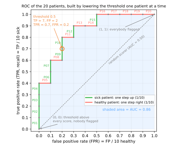
Nesta aula usamos o termo recall, como no scikit-learn e nas saídas do código; é a revocação (sensibilidade) da aula de métricas. Com \(t = 0{,}5\), os 20 pacientes dão TPR = 7/10 = 0,7 e FPR = 2/10 = 0,2: um ponto, \((0{,}2;\ 0{,}7)\). Mude o limiar e o ponto se move. A curva ROC (receiver operating characteristic, nome herdado dos operadores de radar da Segunda Guerra Mundial) é o caminho desse ponto quando o limiar vai de "não sinalizar ninguém" a "sinalizar todo mundo".
2. A curva ROC, à mão
Etapa 1. Eis os 20 pacientes ordenados pelo escore. Com o limiar no escore de um paciente, esse paciente e todos acima dele são sinalizados. Assim, cada linha da tabela é um limiar; as contagens acumuladas de TP e FP dão o ponto:
| paciente | escore | doente | TP | FP | TPR | FPR | precisão |
|---|---|---|---|---|---|---|---|
| — | acima de 0,95 | 0 | 0 | 0,0 | 0,0 | — | |
| P01 | 0,95 | 1 | 1 | 0 | 0,1 | 0,0 | 1,000 |
| P02 | 0,90 | 1 | 2 | 0 | 0,2 | 0,0 | 1,000 |
| P03 | 0,85 | 1 | 3 | 0 | 0,3 | 0,0 | 1,000 |
| P04 | 0,80 | 1 | 4 | 0 | 0,4 | 0,0 | 1,000 |
| P05 | 0,75 | 0 | 4 | 1 | 0,4 | 0,1 | 0,800 |
| P06 | 0,70 | 1 | 5 | 1 | 0,5 | 0,1 | 0,833 |
| P07 | 0,65 | 1 | 6 | 1 | 0,6 | 0,1 | 0,857 |
| P08 | 0,60 | 0 | 6 | 2 | 0,6 | 0,2 | 0,750 |
| P09 | 0,55 | 1 | 7 | 2 | 0,7 | 0,2 | 0,778 |
| P10 | 0,45 | 1 | 8 | 2 | 0,8 | 0,2 | 0,800 |
| P11 | 0,40 | 0 | 8 | 3 | 0,8 | 0,3 | 0,727 |
| P12 | 0,35 | 1 | 9 | 3 | 0,9 | 0,3 | 0,750 |
| P13 | 0,30 | 0 | 9 | 4 | 0,9 | 0,4 | 0,692 |
| P14 | 0,25 | 0 | 9 | 5 | 0,9 | 0,5 | 0,643 |
| P15 | 0,20 | 1 | 10 | 5 | 1,0 | 0,5 | 0,667 |
| P16 | 0,15 | 0 | 10 | 6 | 1,0 | 0,6 | 0,625 |
| P17 | 0,10 | 0 | 10 | 7 | 1,0 | 0,7 | 0,588 |
| P18 | 0,08 | 0 | 10 | 8 | 1,0 | 0,8 | 0,556 |
| P19 | 0,05 | 0 | 10 | 9 | 1,0 | 0,9 | 0,526 |
| P20 | 0,02 | 0 | 10 | 10 | 1,0 | 1,0 | 0,500 |
A regra para desenhá-la é mecânica. Baixar o limiar além de um paciente doente acrescenta um TP: o ponto anda para cima 1/10 (são 10 doentes). Baixá-lo além de um paciente saudável acrescenta um FP: o ponto anda para a direita 1/10 (são 10 saudáveis). O limiar 0,5 da aula de métricas fica entre P09 e P10, na linha de P09: TPR 0,7, FPR 0,2.
Três pontos de referência:
- (0, 0): o limiar está acima de todos os escores, ninguém é sinalizado: nenhum alarme falso e nenhum acerto;
- (1, 1): o limiar está abaixo de todos os escores, todo mundo é sinalizado;
- a diagonal TPR = FPR: um modelo que dá escores aleatórios sinaliza doentes e saudáveis na mesma taxa, qualquer que seja o limiar. Um bom modelo sobe cedo: encontra os doentes primeiro. Um perfeito sobe direto até (0, 1) e depois vai para a direita.
O scikit-learn desenha a mesma curva:
import numpy as np
from sklearn.metrics import roc_curve

score = np.array([0.95, 0.90, 0.85, 0.80, 0.75, 0.70, 0.65, 0.60, 0.55, 0.45,
                  0.40, 0.35, 0.30, 0.25, 0.20, 0.15, 0.10, 0.08, 0.05, 0.02])
sick = np.array([1, 1, 1, 1, 0, 1, 1, 0, 1, 1, 0, 1, 0, 0, 1, 0, 0, 0, 0, 0])

fpr, tpr, thresholds = roc_curve(sick, score)
for t, f, r in zip(thresholds, fpr, tpr):
    print(f"threshold {t:4.2f}   FPR {f:.1f}   TPR {r:.1f}")
_, _, all_thresholds = roc_curve(sick, score, drop_intermediate=False)
print(len(thresholds), "points kept;", len(all_thresholds), "with drop_intermediate=False")
threshold  inf   FPR 0.0   TPR 0.0
threshold 0.95   FPR 0.0   TPR 0.1
threshold 0.80   FPR 0.0   TPR 0.4
threshold 0.75   FPR 0.1   TPR 0.4
threshold 0.65   FPR 0.1   TPR 0.6
threshold 0.60   FPR 0.2   TPR 0.6
threshold 0.45   FPR 0.2   TPR 0.8
threshold 0.40   FPR 0.3   TPR 0.8
threshold 0.35   FPR 0.3   TPR 0.9
threshold 0.25   FPR 0.5   TPR 0.9
threshold 0.20   FPR 0.5   TPR 1.0
threshold 0.02   FPR 1.0   TPR 1.0
12 points kept; 21 with drop_intermediate=False
O primeiro limiar é inf: o canto "não sinalizar ninguém". A lista é mais curta que a tabela porque roc_curve descarta, por padrão (drop_intermediate=True), os pontos no meio de um trecho reto: P02 e P03 estão no segmento de P01 a P04; removê-los não muda a curva. Passe drop_intermediate=False para ter um ponto por escore distinto, mais o canto.
O simulador abaixo faz o mesmo com 600 escores simulados (500 negativos, 100 positivos). Deslize o limiar e veja a matriz de confusão andar ao longo da curva ROC:
3. AUC: um número para a curva inteira
Etapa 2. A área sob a curva ROC (AUC) resume a curva num único número. Para a escada, ela pode ser calculada com retângulos: cada passo para a direita (um paciente saudável) acrescenta um retângulo de largura 1/10 e altura igual à TPR naquele momento. Os pacientes saudáveis aparecem nas alturas 0,4 (P05), 0,6 (P08), 0,8 (P11), 0,9 (P13), 0,9 (P14) e 1,0 (P16 a P20, cinco vezes):
O mesmo número, contado em pares
Agora esqueça a curva. Forme todos os pares (doente, saudável): 10 × 10 = 100 pares. Em quantos o doente recebe o escore maior? Para P05 (0,75), 4 doentes têm escore maior (P01–P04). Para P08, 6. Para P11, 8. Para P13 e P14, 9 cada. Para P16–P20, todos os 10. No total, \(4 + 6 + 8 + 9 + 9 + 5 \times 10 = 86\) dos 100 pares estão na ordem certa: 0,86 de novo.
Não é coincidência. A altura de cada retângulo, vezes 10, é o número de doentes ordenados acima daquele paciente saudável. Logo
com empates contando meio. Esta é a estatística \(U\) de Mann–Whitney dividida pelo número de pares (Hanley & McNeil, 1982); é também a forma mais útil de ler uma AUC: se eu sortear um doente e um saudável, com que frequência o modelo os coloca na ordem certa?
from sklearn.metrics import roc_auc_score

# 1) área: cada paciente saudável soma um retângulo de largura 1/10 e altura = TPR atual
tpr_now, area = 0.0, 0.0
for s in sick:
    if s == 1:
        tpr_now += 1 / 10
    else:
        area += (1 / 10) * tpr_now
# 2) pares: em quantos pares (doente, saudável) o doente tem o escore maior?
pos, neg = score[sick == 1], score[sick == 0]
concordant = (pos[:, None] > neg[None, :]).sum()
print(f"area by rectangles: {area:.2f}")
print(f"concordant pairs:   {concordant} of {len(pos) * len(neg)} = {concordant / (len(pos) * len(neg)):.2f}")
print(f"roc_auc_score:      {roc_auc_score(sick, score):.2f}")
Lendo a escala: AUC = 0,5 é uma ordenação aleatória (a diagonal), AUC = 1 coloca todo doente acima de todo saudável e AUC < 0,5 quer dizer que a ordenação está invertida, errando mais do que acertando. Uma AUC de 0,14 não é um modelo ruim, é um bom modelo com os rótulos trocados: inverta os escores e ele tem 0,86.
O que a AUC mede: a separação entre as classes
A leitura em pares diz o que a AUC mede: o quanto as distribuições de escore dos doentes e dos saudáveis se sobrepõem. Na figura, os saudáveis recebem escores de uma normal \(N(0, 1)\) e os doentes de uma \(N(d, 1)\). Com as classes quase sobrepostas (\(d = 0{,}5\)), sortear um doente e um saudável e perguntar quem tem o escore maior é pouco melhor que jogar uma moeda: AUC 0,64. À medida que as distribuições se afastam, a curva sobe para o canto superior esquerdo e a AUC vai a 0,85 e a 0,98.
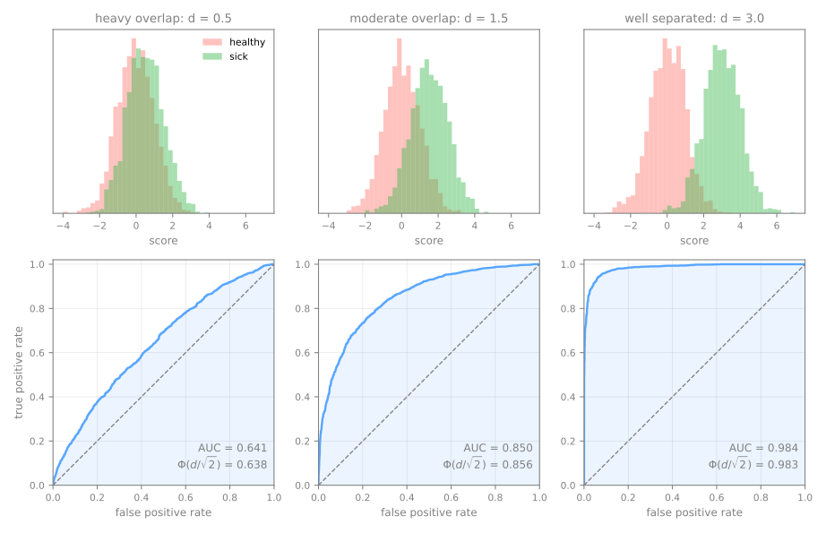
Neste modelo existe até uma fórmula. A diferença entre o escore de um doente e o de um saudável é uma normal \(N(d, 2)\), então \(\text{AUC} = P(\text{diferença} > 0) = \Phi(d/\sqrt{2})\), em que \(\Phi\) é a função de distribuição acumulada da normal padrão:
from scipy.stats import norm

rng = np.random.default_rng(0)
for d in [0.5, 1.5, 3.0]:
    neg, pos = rng.normal(0, 1, 2000), rng.normal(d, 1, 2000)    # saudáveis e doentes
    y, s = np.r_[np.zeros(2000), np.ones(2000)], np.r_[neg, pos]
    print(f"d = {d}: AUC {roc_auc_score(y, s):.3f} · Phi(d / sqrt 2) {norm.cdf(d / np.sqrt(2)):.3f}")
d = 0.5: AUC 0.641 · Phi(d / sqrt 2) 0.638
d = 1.5: AUC 0.850 · Phi(d / sqrt 2) 0.856
d = 3.0: AUC 0.984 · Phi(d / sqrt 2) 0.983
A amostra de 2.000 pacientes por classe fica a menos de 0,01 da fórmula. A lição vale para qualquer modelo: nenhum limiar separa duas distribuições sobrepostas. Mover o limiar só escolhe em que ponto da mesma curva operar; para subir a curva é preciso um modelo, ou atributos, que afaste as distribuições.
Só a ordem importa
Como a AUC conta pares na ordem certa, ela depende apenas da ordenação dos escores, nunca de seus valores. Qualquer transformação que preserve a ordem preserva a AUC:
for name, s in [('score', score), ('score ** 2', score ** 2), ('log(score)', np.log(score)),
                ('100 * score - 7', 100 * score - 7), ('1 - score', 1 - score)]:
    print(f"{name:16s} AUC = {roc_auc_score(sick, s):.2f}")
score            AUC = 0.86
score ** 2       AUC = 0.86
log(score)       AUC = 0.86
100 * score - 7  AUC = 0.86
1 - score        AUC = 0.14
Ao quadrado, com logaritmo ou reescaladas, as "probabilidades" deixam de ser probabilidades (100 × escore − 7 vai até 88), mas a AUC fica em 0,86. Inverter a ordem (1 - score) dá 1 − 0,86 = 0,14. Isso tem duas consequências que vale guardar:
- a AUC não diz nada sobre calibração. Um modelo cujas "probabilidades" estão todas entre 0,40 e 0,41 pode ter AUC 0,99, desde que a ordem esteja certa;
- a AUC não diz nada sobre um limiar em particular. Ela faz uma média sobre todos eles, inclusive limiares que você nunca usaria. Dois modelos com a mesma AUC podem ser muito diferentes no único ponto de operação que importa para você.
Escores, não rótulos
roc_auc_score precisa dos escores: predict_proba(X)[:, 1] ou decision_function(X). Passar a saída de predict é um erro comum que não dispara nenhuma exceção:
from sklearn.metrics import balanced_accuracy_score

labels = (score >= 0.5).astype(int)              # rótulos previstos, não escores
print(f"AUC from labels:   {roc_auc_score(sick, labels):.2f}")   # errado: rótulos
print(f"balanced accuracy: {balanced_accuracy_score(sick, labels):.2f}")
print(f"AUC from scores:   {roc_auc_score(sick, score):.2f}")    # certo: escores
Com apenas dois valores distintos, a "curva" tem um único ponto, (0,2; 0,7), ligado aos cantos por retas. Sua área é \((\text{TPR} + \text{TNR})/2 = (0{,}7 + 0{,}8)/2 = 0{,}75\): a acurácia balanceada em 0,5, não a AUC do modelo, que com os escores dá 0,86. Uma versão mais branda do mesmo efeito aparece com o k-NN: com \(k = 5\), predict_proba só pode assumir os valores 0; 0,2; 0,4; 0,6; 0,8 e 1, então sua curva ROC tem no máximo 7 pontos, uma escada grosseira. O lab avançado mostra uma.
4. A curva precisão–recall
Etapa 3. A curva ROC olha as duas classes separadamente: TPR dentro dos doentes, FPR dentro dos saudáveis. A pergunta que um médico faz quando um paciente é sinalizado é outra: dos pacientes que eu sinalizo, quantos estão mesmo doentes? Essa é a precisão, \(TP / (TP + FP)\), a última coluna da tabela. Plotar a precisão contra o recall (= TPR) para cada limiar dá a curva precisão–recall (PR).
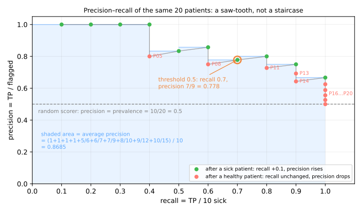
Ela não se parece com a escada ROC. Cada doente move o ponto para a direita (recall + 0,1) e um pouco para cima, porque um alarme correto aumenta a precisão. Cada saudável deixa o recall igual e empurra a precisão para baixo. O resultado é um dente de serra. O ponto final é sempre recall 1 com precisão = 10/20 = 0,5, a fração de doentes entre os 20. Essa fração, a prevalência, é também a curva de um modelo aleatório: se o grupo sinalizado é uma amostra aleatória, sua fração de doentes é a da população, qualquer que seja o limiar. No gráfico PR, a linha "sem habilidade" é, portanto, uma horizontal na altura da prevalência, não uma diagonal.
Precisão média
A curva PR é resumida pela precisão média (AP, average precision):
uma soma, sobre os limiares, do ganho de recall vezes a precisão alcançada ali. O recall só cresce nos doentes, de 1/10 a cada vez, então a AP é simplesmente a média da precisão na posição de cada doente. Pela tabela, essas precisões são 1, 1, 1, 1, 5/6, 6/7, 7/9, 8/10, 9/12 e 10/15:
from sklearn.metrics import auc, average_precision_score, precision_recall_curve

flagged = np.arange(1, 21)                      # limiar no paciente k sinaliza k pacientes
precision_k = np.cumsum(sick) / flagged
print("precision at each sick patient:", precision_k[sick == 1].round(3))
print(f"AP by hand:              {precision_k[sick == 1].mean():.4f}")
print(f"average_precision_score: {average_precision_score(sick, score):.4f}")
prec, rec, _ = precision_recall_curve(sick, score)
print(f"trapezoidal area:        {auc(rec, prec):.4f}")
precision at each sick patient: [1.    1.    1.    1.    0.833 0.857 0.778 0.8   0.75  0.667]
AP by hand:              0.8685
average_precision_score: 0.8685
trapezoidal area:        0.8608
A última linha é uma armadilha a evitar. auc(recall, precision) liga os pontos PR por retas e calcula a área dos trapézios, aqui 0,8608. Mas, entre dois pontos de operação, a precisão não varia linearmente com o recall; a reta descreve classificadores que não existem e o trapézio pode ser otimista (Davis & Goadrich, 2006). A AP soma retângulos, sem interpolar. Os dois números são próximos aqui e podem ficar bem distantes em curvas reais; reporte a AP, calculada com average_precision_score.
5. ROC vs PR quando a classe positiva é rara
As duas curvas reagem de forma diferente a uma coisa: a prevalência. Para isolá-la, mantenha o modelo fixo: pacientes saudáveis recebem escores de uma normal \(N(0, 1)\), doentes de uma \(N(2, 1)\). Depois mude apenas quantos doentes existem, de 50% até 1%:
rng = np.random.default_rng(0)
neg = rng.normal(0, 1, 100_000)                   # saudáveis: escore ~ N(0, 1)
for prev in [0.5, 0.1, 0.01]:
    n_pos = round(len(neg) * prev / (1 - prev))
    pos = rng.normal(2, 1, n_pos)                 # doentes: escore ~ N(2, 1), sempre o mesmo escorador
    s = np.r_[pos, neg]
    y = np.r_[np.ones(n_pos), np.zeros(len(neg))]
    tp, fp = (pos >= 1.16).sum(), (neg >= 1.16).sum()      # um limiar fixo
    print(f"prevalence {prev:4.0%}  AUC {roc_auc_score(y, s):.3f}  AP {average_precision_score(y, s):.3f}"
          f"   at 1.16: TPR {tp / n_pos:.2f}  FPR {fp / len(neg):.2f}  precision {tp / (tp + fp):.2f}")
prevalence  50%  AUC 0.921  AP 0.922   at 1.16: TPR 0.80  FPR 0.12  precision 0.87
prevalence  10%  AUC 0.922  AP 0.666   at 1.16: TPR 0.80  FPR 0.12  precision 0.42
prevalence   1%  AUC 0.914  AP 0.252   at 1.16: TPR 0.79  FPR 0.12  precision 0.06
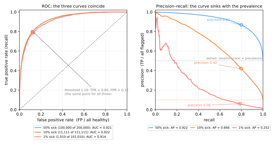
As curvas ROC são a mesma curva (a pequena oscilação da curva de 1% é ruído de amostragem, com apenas 1.010 doentes). As curvas PR desabam: a AP vai de 0,922 para 0,666 e para 0,252. No mesmo limiar, pegando os mesmos cerca de 80% dos doentes com a mesma taxa de 12% de alarmes falsos, a precisão cai de 0,87 para 0,42 e para 0,06. Com prevalência de 1%, 94 de cada 100 pacientes sinalizados são saudáveis.
A razão está nos denominadores. A FPR divide pelo número de saudáveis, então é uma propriedade do modelo só nos saudáveis, cega para quantos doentes existem. A precisão divide pelo número de sinalizados, que mistura as duas classes na proporção de seus tamanhos. Para ver isso, escreva a precisão em termos da prevalência \(\pi\), a fração de doentes na população. Em \(N\) pessoas há \(\pi N\) doentes e \((1-\pi) N\) saudáveis. O modelo sinaliza a fração TPR dos doentes, \(TP = \text{TPR} \cdot \pi N\), e a fração FPR dos saudáveis, \(FP = \text{FPR} \cdot (1-\pi) N\). Na precisão, \(TP / (TP + FP)\), o \(N\) cancela:
TPR e FPR são do modelo; \(\pi\) é da população. Com TPR 0,80 e FPR 0,12: em \(\pi = 0{,}5\), a fórmula dá \(0{,}40 / (0{,}40 + 0{,}06) = 0{,}87\); em \(\pi = 0{,}01\), \(0{,}008 / (0{,}008 + 0{,}119) = 0{,}06\). Uma taxa de alarmes falsos de 12% parece pequena, mas 12% de 100.000 pessoas saudáveis são 12.000 alarmes falsos contra cerca de 800 verdadeiros.
Nenhuma das curvas está errada; elas respondem a perguntas diferentes. Uma regra prática (Saito & Rehmsmeier, 2015):
- ROC / AUC quando as duas classes importam, quando a prevalência em produção é desconhecida ou vai mudar ou quando você compara ordenadores em conjuntos com prevalências diferentes. Ela é livre de prevalência por construção;
- PR / AP quando a classe positiva é rara e o que você paga são os casos sinalizados (alertas a revisar, pacientes a chamar de volta, transações a bloquear). Ela mostra o custo dos alarmes falsos que a curva ROC esconde. Leia a AP sempre contra sua linha de base: uma AP de 0,25 é fraca com prevalência de 50% e 25 vezes melhor que o acaso com 1%.
6. Escolhendo o limiar de operação
Etapa 4. As curvas descrevem todos os limiares; um modelo em produção usa um. Escolhê-lo é uma decisão, então segue a regra usada desde a aula de k-NN para escolher o k: ela é tomada num conjunto de validação, nunca no de teste. (A validação cruzada vai tornar essa escolha mais robusta mais adiante; aqui usamos uma única divisão hold-out.) Trate os 20 pacientes como nosso conjunto de validação e avalie cada limiar segundo quatro critérios comuns:
import pandas as pd

rows = []
for t in score:                                  # o escore de cada paciente é um limiar candidato
    flag = score >= t
    TP = int((flag & (sick == 1)).sum())
    FP = int((flag & (sick == 0)).sum())
    FN = 10 - TP
    rows.append(dict(t=t, TP=TP, FP=FP, precision=TP / (TP + FP), recall=TP / 10,
                     F1=2 * TP / (2 * TP + FP + FN), J=(TP - FP) / 10, cost=10 * FN + FP))
table = pd.DataFrame(rows)
print(table.round(3).to_string(index=False))
   t  TP  FP  precision  recall    F1   J  cost
0.95   1   0      1.000     0.1 0.182 0.1    90
0.90   2   0      1.000     0.2 0.333 0.2    80
0.85   3   0      1.000     0.3 0.462 0.3    70
0.80   4   0      1.000     0.4 0.571 0.4    60
0.75   4   1      0.800     0.4 0.533 0.3    61
0.70   5   1      0.833     0.5 0.625 0.4    51
0.65   6   1      0.857     0.6 0.706 0.5    41
0.60   6   2      0.750     0.6 0.667 0.4    42
0.55   7   2      0.778     0.7 0.737 0.5    32
0.45   8   2      0.800     0.8 0.800 0.6    22
0.40   8   3      0.727     0.8 0.762 0.5    23
0.35   9   3      0.750     0.9 0.818 0.6    13
0.30   9   4      0.692     0.9 0.783 0.5    14
0.25   9   5      0.643     0.9 0.750 0.4    15
0.20  10   5      0.667     1.0 0.800 0.5     5
0.15  10   6      0.625     1.0 0.769 0.4     6
0.10  10   7      0.588     1.0 0.741 0.3     7
0.08  10   8      0.556     1.0 0.714 0.2     8
0.05  10   9      0.526     1.0 0.690 0.1     9
0.02  10  10      0.500     1.0 0.667 0.0    10
print("max F1:              t =", table.loc[table.F1.idxmax(), 't'])
print("max Youden J:        t =", table.loc[table.J == table.J.max(), 't'].tolist())
ok = table[table.recall >= 0.9]
print("recall >= 0.9, best precision: t =", ok.loc[ok.precision.idxmax(), 't'])
print("min cost (FN = 10 FP): t =", table.loc[table.cost.idxmin(), 't'], "  cost", table.cost.min())
max F1:              t = 0.35
max Youden J:        t = [0.45, 0.35]
recall >= 0.9, best precision: t = 0.35
min cost (FN = 10 FP): t = 0.2   cost 5
Quatro critérios, nem todos com a mesma resposta:
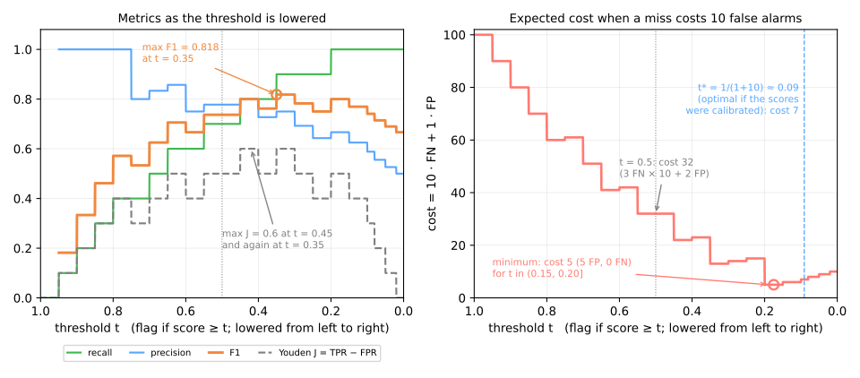
- F1 máximo escolhe \(t = 0{,}35\): 9 de 10 doentes encontrados, 3 alarmes falsos, F1 = 0,818. O F1 pesa precisão e recall igualmente, o que raramente é o que a aplicação quer, mas é um padrão razoável quando ninguém sabe dizer outra coisa.
- O J de Youden \(= \text{TPR} - \text{FPR}\) (Youden, 1950) é a distância vertical do ponto ROC até a diagonal. Aqui ele empata em 0,6 entre \(t = 0{,}45\) (TPR 0,8, FPR 0,2) e \(t = 0{,}35\) (TPR 0,9, FPR 0,3). Ele ignora a prevalência, como a curva ROC em que vive.
- "Recall ≥ 0,9, depois a melhor precisão" é como os requisitos costumam chegar ("temos de pegar pelo menos 90% dos casos"): entre os limiares que chegam a recall 0,9, \(t = 0{,}35\) tem a melhor precisão, 0,75.
- Custo esperado mínimo. Suponha que deixar passar uma doença custe 10 vezes mais que um encaminhamento desnecessário: custo = 10·FN + 1·FP. O mínimo, custo 5, está em \(t = 0{,}20\): os 10 doentes encontrados, 5 saudáveis encaminhados. O padrão 0,5 custa 32 (3 perdas × 10 + 2 alarmes falsos).
Para o critério de custo existe também uma fórmula. Se os escores fossem probabilidades calibradas, sinalizar um paciente com probabilidade \(p\) custaria \((1-p)\,c_{FP}\) em média; não sinalizar custaria \(p\,c_{FN}\). Sinalize quando o segundo for maior:
(Elkan, 2001). Nos nossos 20 pacientes, \(t = 0{,}10\) custa 7 (7 alarmes falsos, nenhuma perda), perto do mínimo empírico mas não igual: nossos escores não são perfeitamente calibrados e 20 pacientes é uma amostra pequena. A fórmula diz onde procurar; o conjunto de validação diz onde parar. Note também que 0,5 é o limiar certo apenas quando os dois erros custam o mesmo e os escores são calibrados. Fora disso, nada no 0,5 é especial.
O scikit-learn (≥ 1.5) automatiza isso com TunedThresholdClassifierCV, que procura o limiar por validação cruzada segundo o critério que você passar em scoring (por padrão, a acurácia balanceada, isto é, o J de Youden). Você poderá usá-lo depois da aula de validação cruzada; o procedimento é o mesmo que fizemos à mão nesta seção.
Ideia-chave
A curva é o modelo; o ponto sobre ela é a sua decisão. A AUC e a AP avaliam a ordenação, que o treino produz; o limiar escolhe o ponto de operação, que você produz — e que pode ser mudado depois, sem retreinar nada.
7. Resumo: as duas curvas e o ponto de operação
| curva ROC | curva precisão–recall | |
|---|---|---|
| eixos | FPR × TPR | recall × precisão |
| denominadores | cada classe separadamente | a coluna dos sinalizados, que mistura as duas |
| linha "sem habilidade" | a diagonal | uma horizontal na prevalência |
| número que a resume | AUC = P(doente ordenado acima de saudável) | AP = média da precisão em cada positivo |
| muda com a prevalência? | não | sim |
| use quando | as duas classes importam; a prevalência vai mudar | a classe positiva é rara e você paga pelos casos sinalizados |
- Avalie a ordenação com AUC e AP, sempre passando escores, nunca rótulos.
- Leia a AP contra a prevalência: 0,25 é fraco com 50% de positivos e 25 vezes melhor que o acaso com 1%.
- Escolha o limiar na validação, por um critério declarado: uma meta de recall, uma razão de custos, o melhor F1 se nada mais for conhecido.
- Nada no 0,5 é especial fora do caso em que os dois erros custam o mesmo e os escores são calibrados.
Lab fundamental — as curvas de uma triagem
O conjunto mammography (OpenML 310, também um dos benchmarks do artigo do SMOTE) tem 11.183 regiões de mamografias descritas por 6 atributos numéricos calculados a partir da imagem, das quais 260 (2,3%) são microcalcificações, pequenos depósitos de cálcio que podem ser um sinal precoce de câncer de mama. Daqui em diante, elas são a classe positiva, chamada de maligna para abreviar; o resto é benigna. A tarefa: sinalizá-las para um radiologista olhar. Deixar passar uma é muito pior do que um alarme falso, então a meta é declarada de saída: recall de pelo menos 0,80 nos casos malignos, com a melhor precisão possível.
Como fazer este lab em aula (cerca de 35 min, em duplas)
- Abra o notebook do lab no Colab. Não é preciso baixar nem instalar nada: o Colab roda no navegador. Para guardar as suas respostas, salve uma cópia no seu Drive (Arquivo → Salvar uma cópia no Drive) antes de editar. Rode as células em ordem, numa mesma sessão.
- Este lab corresponde aos passos 1 a 5 do notebook. O lab avançado continua no mesmo notebook, a partir do passo 6.
- Cada passo começa com um Preveja: responda com a dupla antes de rodar a célula. Errar a previsão é o que torna o resultado memorável.
- Depois de rodar, compare com a saída e a leitura desta página. Toda saída aqui é exatamente o que o código imprime.
- As Simulações pedem que vocês escrevam um pequeno experimento em Python: mudar uma entrada e observar o que acontece com a saída. Nada de conta à mão. A solução fica recolhida logo abaixo: tente antes de abrir.
- Ritmo sugerido: passos 1 a 3 em 10 min; passo 4 e a simulação em 12 min; passo 5 e a simulação em 13 min.
Passo 1 — carregar e olhar a prevalência
Preveja. Microcalcificações são achados raros numa mamografia. Antes de rodar: você espera que elas sejam mais ou menos de 10% das regiões? Com essa prevalência, quanto de acurácia um modelo que nunca sinaliza nada conseguiria?
import numpy as np
import pandas as pd
from sklearn.datasets import fetch_openml

mammo = fetch_openml(data_id=310, as_frame=True)
X = mammo.data                                   # 6 atributos numéricos por região
y = (mammo.target == '1').astype(int)            # o alvo é '-1' (benigno) ou '1' (maligno)
print(X.shape)
print(y.value_counts())
print(f"prevalence: {y.mean():.2%}")
O alvo vem como as strings '-1' e '1'; nós o mapeamos para 0/1 de modo que 1 seja a classe que queremos pegar. 260 das 11.183 regiões são malignas: 2,32%. Toda métrica que calcularmos tem de ser lida contra esse número.
Passo 2 — divisão estratificada treino / validação / teste
Preveja. Por que estratificar importa mais aqui do que num conjunto equilibrado? Se a validação tiver cerca de 50 casos malignos, quanto de recall vale um único caso?
from sklearn.model_selection import train_test_split

X_tmp, X_test, y_tmp, y_test = train_test_split(X, y, test_size=0.2, stratify=y, random_state=7)
X_train, X_val, y_train, y_val = train_test_split(X_tmp, y_tmp, test_size=0.25,
                                                  stratify=y_tmp, random_state=7)
for name, part in [('train', y_train), ('validation', y_val), ('test', y_test)]:
    print(f"{name:10s} {len(part):5d} rows  {part.sum():3d} malignant  ({part.mean():.2%})")
train       6709 rows  156 malignant  (2.33%)
validation  2237 rows   52 malignant  (2.32%)
test        2237 rows   52 malignant  (2.32%)
60/20/20, estratificada. O treino ajusta os modelos e a validação escolhe entre eles e fixa o limiar; o conjunto de teste é usado uma vez, no passo 10. Repare como cada parte tem poucos positivos: 52 casos malignos na validação significam que um caso vale quase 2 pontos de recall.
Passo 3 — um baseline que nunca sinaliza nada
Preveja. Qual vai ser a acurácia de responder "benigno" para todas as regiões? E o recall?
from sklearn.dummy import DummyClassifier
from sklearn.metrics import accuracy_score, recall_score

dummy = DummyClassifier(strategy='most_frequent').fit(X_train, y_train)
pred = dummy.predict(X_val)
print(f"accuracy {accuracy_score(y_val, pred):.4f}   recall {recall_score(y_val, pred):.3f}")
Responder "benigno" para tudo dá 97,7% de acurácia e não encontra nenhum câncer. É com essa marca que a acurácia precisa ser comparada; é por isso que não vamos mais olhar para ela.
Passo 4 — uma regressão logística no limiar padrão
Preveja. A acurácia vai superar a do baseline por muito ou por pouco? E o recall em 0,5: você espera perto de 0,9 ou bem abaixo disso, dado que só 2,3% das regiões são malignas?
from sklearn.linear_model import LogisticRegression
from sklearn.metrics import average_precision_score, precision_score, roc_auc_score
from sklearn.pipeline import make_pipeline
from sklearn.preprocessing import StandardScaler

lr = make_pipeline(StandardScaler(), LogisticRegression()).fit(X_train, y_train)
p_val = lr.predict_proba(X_val)[:, 1]
pred = (p_val >= 0.5).astype(int)
print(f"accuracy {accuracy_score(y_val, pred):.4f}   flagged {pred.sum()} of {len(pred)}")
print(f"recall {recall_score(y_val, pred):.3f}   precision {precision_score(y_val, pred):.3f}")
print(f"ROC AUC {roc_auc_score(y_val, p_val):.3f}   AP {average_precision_score(y_val, p_val):.3f}"
      f"   (AP of a random scorer = {y_val.mean():.3f})")
accuracy 0.9839   flagged 30 of 2237
recall 0.442   precision 0.767
ROC AUC 0.946   AP 0.653   (AP of a random scorer = 0.023)
Como ler:
- acurácia de 98,4%, mal acima dos 97,7% do dummy;
- em 0,5 o modelo sinaliza só 30 regiões: 23 delas são malignas (precisão 0,767), mas são 23 de 52, recall 0,442. Mais da metade dos cânceres passa, longe da meta de 0,80;
- a ordenação é boa: ROC AUC 0,946 e AP 0,653, contra uma AP de 0,023 de um modelo aleatório (cerca de 28 vezes melhor). O modelo sabe bastante; 0,5 é só o corte errado para este problema.
Simulação: a AUC só enxerga a ordem. Pegue os escores p_val e transforme-os de maneiras que preservam a ordem (elevar ao cubo, virar chances \(p/(1-p)\)) e de uma que a inverte (\(1-p\)). Para cada versão, meça a AUC, a AP e quantas regiões ficam acima de 0,5. O que muda e o que não muda?
Solução
for name, s in [('p', p_val), ('p ** 3', p_val ** 3),
                ('p / (1 - p)', p_val / (1 - p_val)), ('1 - p', 1 - p_val)]:
    flagged = (s >= 0.5).sum()
    print(f"{name:12s} AUC {roc_auc_score(y_val, s):.3f}   AP {average_precision_score(y_val, s):.3f}"
          f"   sinalizadas em 0,5: {flagged:4d}   recall {recall_score(y_val, s >= 0.5):.3f}")
p            AUC 0.946   AP 0.653   sinalizadas em 0,5:   30   recall 0.442
p ** 3       AUC 0.946   AP 0.653   sinalizadas em 0,5:   14   recall 0.231
p / (1 - p)  AUC 0.946   AP 0.653   sinalizadas em 0,5:   38   recall 0.558
1 - p        AUC 0.054   AP 0.012   sinalizadas em 0,5: 2207   recall 0.558
As três primeiras linhas têm exatamente a mesma AUC e a mesma AP, porque nenhuma transformação crescente muda quem vem antes de quem. O que muda, e muito, é o ponto de operação em 0,5: de 14 a 38 regiões sinalizadas, com o recall indo de 0,231 a 0,558. Ou seja, a AUC avalia o que o treino produziu (a ordenação) e é cega para o corte; o 0,5, por sua vez, só significa alguma coisa se os escores forem probabilidades de verdade. A última linha inverte a ordem: a AUC vira \(1 - 0{,}946 = 0{,}054\), um "modelo péssimo" que na verdade é o mesmo modelo com o sinal trocado.
Passo 5 — as curvas ROC e PR
Preveja. Para chegar a recall 0,80 neste conjunto, você acha que a precisão fica mais perto de 0,8 ou de 0,3? Lembre que só 2,3% das regiões são malignas.
import matplotlib.pyplot as plt
from sklearn.metrics import PrecisionRecallDisplay, RocCurveDisplay, precision_recall_curve, roc_curve

fig, (ax1, ax2) = plt.subplots(1, 2, figsize=(10, 4))
RocCurveDisplay.from_predictions(y_val, p_val, ax=ax1, plot_chance_level=True)
PrecisionRecallDisplay.from_predictions(y_val, p_val, ax=ax2, plot_chance_level=True)
plt.show()

fpr, tpr, _ = roc_curve(y_val, p_val)
for max_fpr in [0.01, 0.05, 0.10]:
    print(f"FPR <= {max_fpr:.2f}: best recall {tpr[fpr <= max_fpr].max():.3f}")
prec, rec, _ = precision_recall_curve(y_val, p_val)
for min_rec in [0.5, 0.8, 0.9]:
    print(f"recall >= {min_rec:.1f}: best precision {prec[rec >= min_rec].max():.3f}")
FPR <= 0.01: best recall 0.654
FPR <= 0.05: best recall 0.808
FPR <= 0.10: best recall 0.904
recall >= 0.5: best precision 0.784
recall >= 0.8: best precision 0.294
recall >= 0.9: best precision 0.232
Os dois gráficos mostram o mesmo modelo. A curva ROC sobe rápido: com taxa de falsos positivos de 5% ela já chega a recall 0,808. Parece barato, mas 5% das 2.185 regiões benignas são até 109 alarmes falsos, contra 42 cânceres encontrados. A curva PR mostra esse preço diretamente: para chegar a recall 0,8 a melhor precisão é 0,294, ou seja, cerca de 2 de cada 3 regiões sinalizadas são benignas; para chegar a 0,9 ela cai para 0,232. Esse é o compromisso com que os radiologistas vão conviver e nenhuma das curvas pode mudá-lo. Só a escolha do ponto sobre a curva é nossa.
Simulação: o preço de cada ponto de recall. Para metas de recall de 0,50 a 0,95, encontre na validação o limiar que atinge a meta com a melhor precisão e conte quantas regiões ele sinaliza. Traduza a precisão em algo que um radiologista entenda: quantas regiões benignas ele revisa para cada câncer encontrado?
Solução
prec, rec, thr = precision_recall_curve(y_val, p_val)
print("meta   limiar  sinalizadas  precisão  benignas revistas por câncer encontrado")
for meta in [0.5, 0.7, 0.8, 0.9, 0.95]:
    ok = rec[:-1] >= meta
    i = int(np.argmax(np.where(ok, prec[:-1], -1)))
    flag = p_val >= thr[i]
    tp = int((flag & (y_val == 1)).sum()); fp = int((flag & (y_val == 0)).sum())
    print(f"{meta:4.2f}   {thr[i]:6.4f}  {flag.sum():11d}  {prec[i]:8.3f}  {fp / tp:34.1f}")
meta   limiar  sinalizadas  precisão  benignas revistas por câncer encontrado
0.50   0.3651           37     0.784                                 0.3
0.70   0.1085           82     0.451                                 1.2
0.80   0.0632          143     0.294                                 2.4
0.90   0.0425          203     0.232                                 3.3
0.95   0.0050          835     0.060                                15.7
A última coluna é a curva PR escrita como carga de trabalho. Com meta de recall 0,50, o radiologista revisa uma região benigna a cada três cânceres; subindo para 0,80, passa a revisar quase duas e meia por câncer; em 0,95, quase 16. O custo de cada ponto extra de recall cresce rápido e é por isso que a meta de 0,80 foi declarada antes de ver os dados em vez de depois. Repare também que o limiar correspondente desce de 0,37 para 0,005: nada nesses números se parece com 0,5.
Para fechar a parte fundamental. Em uma frase cada: (1) por que a curva ROC não muda quando a doença fica mais rara e a curva PR muda? (2) O que a AUC mede que a acurácia em 0,5 não mede? (3) Quem decide o ponto de operação, o treino ou você?
Sua vez (fundamental)
Para casa:
- A escada à mão. Pegue os 10 primeiros pacientes do exemplo das 20 linhas e desenhe a curva ROC deles no papel, um degrau por paciente. Confira com
roc_curve. Em que ponto está o limiar 0,5? - AUC sem calibração. Comprima os escores da validação do passo 4 para a faixa de 0,40 a 0,41 com
0.40 + 0.01 * p_val. O que acontece com a AUC e o que acontece com a acurácia em 0,5? Que métrica você usaria para descobrir que as probabilidades estão erradas? - AP contra a linha de base. Calcule a AP de um escorador aleatório (use
rng.random(len(y_val))) e compare com a AP do modelo e com a prevalência. Quantas vezes melhor que o acaso o modelo é?
Abordagem avançada
A parte fundamental tratou de avaliar e cortar uma ordenação. Esta parte vai ao cenário em que isso mais importa: a classe de interesse é 2% das linhas. A pergunta passa a ser o que de fato muda quando aplicamos os remédios comuns — pesos de classe, reamostragem, SMOTE — e o que eles não mudam. Os blocos de código continuam os das seções 1 a 6 (o código dos labs roda à parte, no Colab): os imports e os 20 pacientes (score, sick) já estão na sessão.
Esta parte termina com uma ordem de ataque e, antes dela, segue quatro etapas, desenhadas abaixo: 1. o que dá errado quando a classe é rara; 2. três remédios: pesos de classe, limiar deslocado, reamostragem; 3. lado a lado, na mesma divisão; 4. duas armadilhas que fazem um remédio parecer melhor do que é. Cada etapa leva à sua seção e, nos slides, uma faixa embaixo mostra em que etapa você está.
- O que dá errado2% de fraude: acurácia alta, recall baixo; o problema é o modelo ou o limiar?
- Três remédiospesos de classe, limiar deslocado, reamostragem e SMOTE
- Lado a ladocinco abordagens na mesma divisão, uma curva só
- Duas armadilhasreamostrar antes da divisão; probabilidades distorcidas
Slides da abordagem avançada
Clique nos slides e use as setas ← → para navegar; F abre em tela cheia e Esc mostra todos os slides. Abrir os slides numa aba nova
8. Dados desbalanceados: o que dá errado
Etapa 1. Agora o lado do treino. Tome uma triagem de fraude simulada: 20.000 transações de cartão, cerca de 2% fraudulentas, 5 atributos numéricos que são um pouco maiores, em média, nas fraudes. A divisão é 60/20/20 com stratify=y, então cada parte mantém os 2%:
from sklearn.model_selection import train_test_split

rng = np.random.default_rng(0)
n = 20_000
y = (rng.random(n) < 0.02).astype(int)                               # cerca de 2% de fraude
X = rng.normal(size=(n, 5)) + y[:, None] * np.array([1.2, 1.0, 0.8, 0.8, 0.6])

X_tmp, X_test, y_tmp, y_test = train_test_split(X, y, test_size=0.2, stratify=y, random_state=0)
X_train, X_val, y_train, y_val = train_test_split(X_tmp, y_tmp, test_size=0.25,
                                                  stratify=y_tmp, random_state=0)
for name, part in [('train', y_train), ('validation', y_val), ('test', y_test)]:
    print(f"{name:10s} {len(part):6,d} rows  {part.sum():4d} frauds  ({part.mean():.2%})")
train      12,000 rows   233 frauds  (1.94%)
validation  4,000 rows    77 frauds  (1.93%)
test        4,000 rows    78 frauds  (1.95%)
Sem stratify, o número de fraudes em cada parte mudaria de divisão para divisão; com tão poucos positivos, só isso já move o recall em vários pontos. Estratificar é o primeiro remédio e é de graça. Uma regressão logística, treinada como de costume:
from sklearn.dummy import DummyClassifier
from sklearn.linear_model import LogisticRegression
from sklearn.metrics import accuracy_score, precision_score, recall_score
from sklearn.pipeline import make_pipeline
from sklearn.preprocessing import StandardScaler

dummy = DummyClassifier(strategy='most_frequent').fit(X_train, y_train)
plain = make_pipeline(StandardScaler(), LogisticRegression()).fit(X_train, y_train)
p_plain = plain.predict_proba(X_test)[:, 1]
pred = plain.predict(X_test)                     # limiar 0.5
print(f"dummy accuracy:   {accuracy_score(y_test, dummy.predict(X_test)):.4f}")
print(f"model accuracy:   {accuracy_score(y_test, pred):.4f}")
print(f"flagged:          {pred.sum()} of {len(pred)}  (true frauds: {y_test.sum()})")
print(f"recall:           {recall_score(y_test, pred):.3f}   precision: {precision_score(y_test, pred):.3f}")
print(f"ROC AUC:          {roc_auc_score(y_test, p_plain):.3f}   AP: {average_precision_score(y_test, p_plain):.3f}")
print(f"mean probability: {p_plain.mean():.4f}   median: {np.median(p_plain):.4f}")
dummy accuracy:   0.9805
model accuracy:   0.9838
flagged:          23 of 4000  (true frauds: 78)
recall:           0.231   precision: 0.783
ROC AUC:          0.930   AP: 0.459
mean probability: 0.0206   median: 0.0030
(Nesta seção o conjunto de teste é só exibido, para comparar os remédios nas mesmas linhas; toda escolha, como um limiar, é feita no conjunto de validação.)
A acurácia, 98,38%, parece excelente e não diz quase nada: o dummy que nunca sinaliza nada já tem 98,05%. O modelo sinaliza 23 transações e pega 18 das 78 fraudes, um recall de 0,23. Mas a ordenação é boa: ROC AUC 0,930. Sorteie uma fraude e uma transação legítima: em 93% das vezes, a fraude recebe o escore maior.
Então o modelo não é cego; suas probabilidades é que são pequenas. A transação mediana recebe 0,003; 60 das 78 fraudes ficam abaixo de 0,5. Isso é honesto: com uma taxa base de 2%, mesmo uma transação suspeita costuma ser mais provavelmente legítima do que não, então poucas passam de 0,5. O problema é o limiar e a métrica, não necessariamente o modelo. Esse diagnóstico importa porque cada remédio abaixo age numa parte diferente: alguns mudam o ponto de operação, outros a ordenação; é fácil confundi-los.
9. Remédios, medidos lado a lado
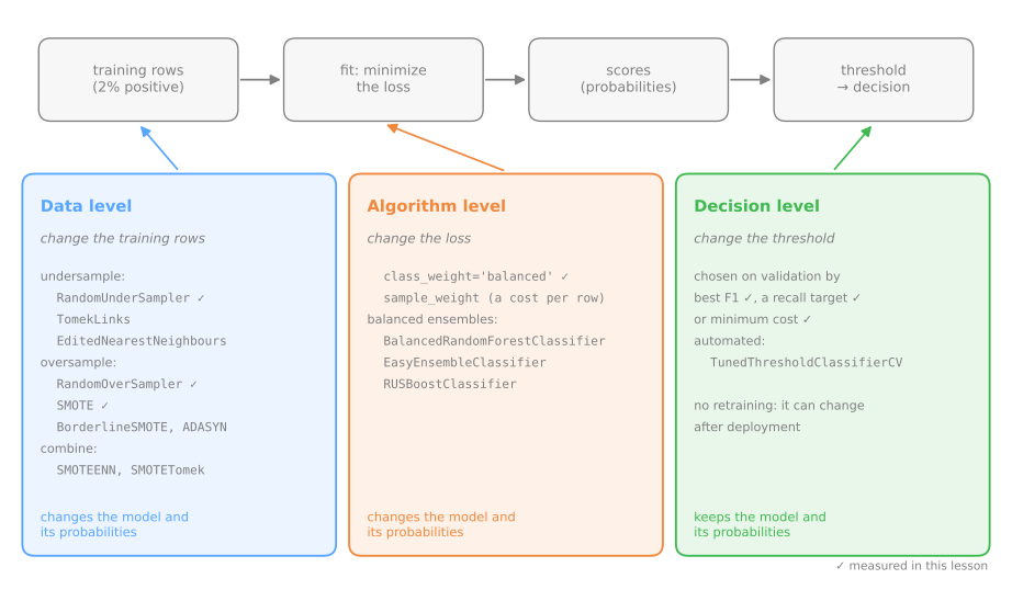
Etapa 2. Três famílias de remédio, medidas na mesma divisão: mudar o peso de cada classe na perda, mudar o limiar e mudar as linhas de treino.
Cada família age num ponto diferente do caminho entre as linhas de treino e a decisão. A figura situa as três e lista também as variantes mais comuns do imblearn que esta aula não mede:
Pesos de classe
A maioria dos classificadores do scikit-learn aceita class_weight. Com 'balanced', cada exemplo da classe \(c\) entra na perda com peso
em que \(n\) é o número de linhas, \(k = 2\) o número de classes e \(n_c\) as linhas da classe \(c\). No nosso conjunto de treino, \(n = 12.000\), com 11.767 legítimas e 233 fraudes: \(w_0 = 12000 / (2 \times 11767) = 0{,}510\) e \(w_1 = 12000 / (2 \times 233) = 25{,}751\). Cada fraude agora pesa tanto quanto 50 transações legítimas: as duas classes contribuem igualmente para a perda.
from sklearn.utils.class_weight import compute_class_weight

n_c = np.bincount(y_train)                       # [legítima, fraude]
print("by hand:", (len(y_train) / (2 * n_c)).round(3))
print("sklearn:", compute_class_weight('balanced', classes=np.array([0, 1]), y=y_train).round(3))
weighted = make_pipeline(StandardScaler(), LogisticRegression(class_weight='balanced'))
weighted.fit(X_train, y_train)
p_w = weighted.predict_proba(X_test)[:, 1]
for name, p in [('no weights', p_plain), ('balanced', p_w)]:
    flag = p >= 0.5
    print(f"{name:10s}  AUC {roc_auc_score(y_test, p):.3f}  AP {average_precision_score(y_test, p):.3f}  "
          f"flagged {flag.sum():3d}  recall {recall_score(y_test, flag):.3f}  "
          f"precision {precision_score(y_test, flag):.3f}")
no weights  AUC 0.930  AP 0.459  flagged  23  recall 0.231  precision 0.783
balanced    AUC 0.929  AP 0.460  flagged 673  recall 0.821  precision 0.095
As métricas de ordenação quase não se movem: AUC 0,930 → 0,929, AP 0,459 → 0,460. O que se move é o ponto de operação em 0,5: 23 → 673 transações sinalizadas, recall 0,231 → 0,821, precisão 0,783 → 0,095. Os pesos não tornaram o modelo melhor em separar fraudes do resto; fizeram-no dizer "fraude" com muito mais frequência.
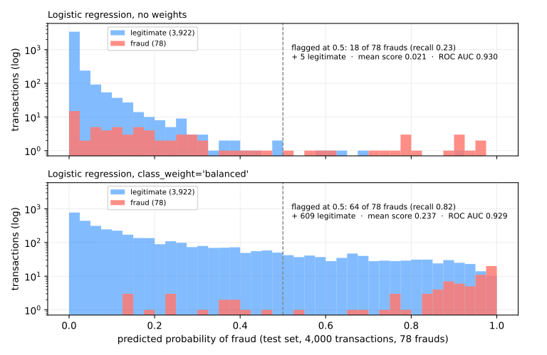
Para a regressão logística podemos ver exatamente como. Compare os parâmetros ajustados:
lr_plain, lr_w = plain[-1], weighted[-1]
print("no weights: coef", lr_plain.coef_[0].round(2), " intercept", lr_plain.intercept_[0].round(2))
print("balanced:   coef", lr_w.coef_[0].round(2), " intercept", lr_w.intercept_[0].round(2))
print(f"intercept shift {lr_w.intercept_[0] - lr_plain.intercept_[0]:.2f}"
      f"   log(n0 / n1) = {np.log(n_c[0] / n_c[1]):.2f}")
no weights: coef [1.07 1.   0.85 0.8  0.59]  intercept -5.77
balanced:   coef [1.09 1.04 0.78 0.84 0.68]  intercept -1.9
intercept shift 3.86   log(n0 / n1) = 3.92
As inclinações ficam a menos de 0,1 umas das outras; o intercepto sobe 3,86, quase exatamente \(\log(n_0/n_1) = \log(11767/233) = 3{,}92\). Pesar os positivos por \(n_0/n_1\) multiplica as chances (odds) por esse fator, o que em log-odds é somar uma constante. Para uma regressão logística, class_weight='balanced' é aproximadamente um intercepto deslocado, que é a mesma coisa que um limiar deslocado.
Movendo o limiar
Se os pesos basicamente movem o limiar, podemos mover o limiar diretamente e manter o modelo sem pesos. Somar \(\log(n_0/n_1)\) às log-odds e cortar em 0,5 é o mesmo que cortar a probabilidade original em \(n_1/(n_0 + n_1)\), a prevalência do treino:
t_prev = y_train.mean()                          # limiar = prevalência do treino
moved = p_plain >= t_prev
print(f"no weights, t = {t_prev:.4f}: flagged {moved.sum()}  recall {recall_score(y_test, moved):.3f}  "
      f"precision {precision_score(y_test, moved):.3f}")
print(f"balanced,   t = 0.5   : flagged {(p_w >= 0.5).sum()}  recall {recall_score(y_test, p_w >= 0.5):.3f}  "
      f"precision {precision_score(y_test, p_w >= 0.5):.3f}")
print("transactions classified differently:", (moved != (p_w >= 0.5)).sum(), "of", len(y_test))
no weights, t = 0.0194: flagged 685  recall 0.833  precision 0.095
balanced,   t = 0.5   : flagged 673  recall 0.821  precision 0.095
transactions classified differently: 42 of 4000
Mesmo ponto de operação, sem retreinar: as duas regras discordam em 42 de 4.000 transações. O limiar também não precisa ser a prevalência. Qualquer critério da seção 6 (melhor F1, uma meta de recall, um custo) pode ser aplicado aos escores de validação do modelo sem pesos. Muitas vezes este é o remédio mais barato e o único que pode ser mudado depois da implantação sem mexer no modelo.
Reamostragem: mudar os dados de treino
A terceira família muda as linhas em que o modelo é treinado, para que as classes pareçam balanceadas. A biblioteca imbalanced-learn (pip install imbalanced-learn, importada como imblearn) oferece os métodos padrão com interface do scikit-learn:
- Subamostragem aleatória (
RandomUnderSampler) descarta linhas da maioria ao acaso até as classes ficarem iguais. Rápida, mas joga informação fora: aqui, 11.534 das 11.767 transações legítimas; - Sobreamostragem aleatória (
RandomOverSampler) duplica linhas da minoria ao acaso. Nada é jogado fora, mas cada fraude se repete cerca de 50 vezes e um modelo flexível pode decorar as cópias; - SMOTE (Synthetic Minority Over-sampling Technique, Chawla et al., 2002) cria pontos novos da minoria. Para um ponto da minoria \(x_i\), ele escolhe um de seus \(k\) vizinhos mais próximos da minoria, \(x_{nn}\) (como no k-NN, padrão \(k = 5\)), sorteia um \(\lambda \in [0, 1]\) e acrescenta
um ponto no segmento entre eles.
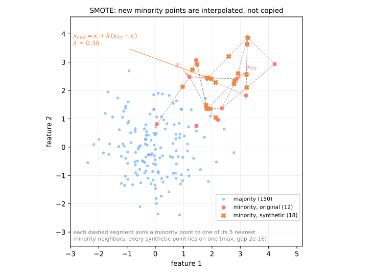
A figura mostra o que o SMOTE faz e sua limitação. Os pontos sintéticos preenchem a região entre os pontos da minoria em vez de se empilharem sobre eles, o que é mais suave que duplicar. Mas o SMOTE só olha vizinhos da minoria: ele traça sem problema um segmento atravessando uma região cheia de pontos da maioria (o ponto da minoria mais abaixo e à esquerda na figura está dentro da nuvem azul; um ponto sintético foi criado no caminho até ele). Variantes como Borderline-SMOTE e SMOTE + ligações de Tomek limpam esses pontos; nenhuma muda a ideia básica.
ferramenta do imblearn | o que faz |
|---|---|
TomekLinks | remove o ponto da maioria de cada par de vizinhos mais próximos mútuos de classes diferentes: limpa a fronteira |
EditedNearestNeighbours | remove pontos da maioria que não concordam com seus 3 vizinhos mais próximos (por padrão, basta um discordar) |
BorderlineSMOTE | aplica o SMOTE só aos pontos da minoria perto da fronteira, cercados em maior parte pela maioria |
ADASYN | gera mais pontos sintéticos em torno dos pontos da minoria com mais vizinhos da maioria, os mais difíceis |
SMOTEENN, SMOTETomek | SMOTE seguido de uma limpeza por ENN ou por ligações de Tomek |
BalancedRandomForestClassifier | uma random forest em que cada árvore treina numa amostra balanceada por subamostragem |
EasyEnsembleClassifier | vários AdaBoost, cada um numa subamostra balanceada diferente da maioria |
RUSBoostClassifier | AdaBoost com subamostragem aleatória antes de cada rodada |
As limpezas (Tomek, ENN) removem poucas linhas e mexem pouco no desbalanceamento; os ensembles balanceados combinam a subamostragem com a média de muitos modelos, o que recupera parte da informação que cada subamostra joga fora. Todas cabem num pipeline do imblearn e devem ser comparadas como as outras: na validação, com a mesma métrica.
A reamostragem só pode tocar os dados de treino. Os conjuntos de validação e teste precisam manter a prevalência real, porque é ela que o modelo vai encontrar. O imblearn.pipeline.Pipeline (ou seu make_pipeline) garante isso: um amostrador dentro dele roda durante o fit e é pulado no predict. Um pipeline comum do sklearn não aceita um amostrador.
from imblearn.over_sampling import SMOTE, RandomOverSampler
from imblearn.pipeline import make_pipeline as make_imb_pipeline
from imblearn.under_sampling import RandomUnderSampler

samplers = {'undersampling': RandomUnderSampler(random_state=0),
            'oversampling': RandomOverSampler(random_state=0),
            'SMOTE': SMOTE(random_state=0)}
for name, sampler in samplers.items():
    X_r, y_r = sampler.fit_resample(X_train, y_train)
    print(f"{name:14s} the model trains on {len(y_r):6,d} rows, {y_r.sum():6,d} of them fraud")
undersampling  the model trains on    466 rows,    233 of them fraud
oversampling   the model trains on 23,534 rows, 11,767 of them fraud
SMOTE          the model trains on 23,534 rows, 11,767 of them fraud
A comparação
Etapa 3. As cinco abordagens na mesma divisão. Para cada uma: as métricas de ordenação, o ponto de operação em 0,5 e o ponto de operação no limiar que maximiza o F1 no conjunto de validação, medido depois no conjunto de teste:
from sklearn.metrics import f1_score

models = {'no weights': make_pipeline(StandardScaler(), LogisticRegression()),
          'balanced weights': make_pipeline(StandardScaler(), LogisticRegression(class_weight='balanced'))}
for name, sampler in samplers.items():
    models[name] = make_imb_pipeline(StandardScaler(), sampler, LogisticRegression())

rows = []
for name, model in models.items():
    model.fit(X_train, y_train)                  # a reamostragem, se houver, acontece aqui, só no X_train
    prec, rec, thr = precision_recall_curve(y_val, model.predict_proba(X_val)[:, 1])
    t_best = thr[np.argmax(2 * prec[:-1] * rec[:-1] / (prec[:-1] + rec[:-1] + 1e-12))]   # na validação
    p = model.predict_proba(X_test)[:, 1]
    row = {'model': name, 'AUC': roc_auc_score(y_test, p), 'AP': average_precision_score(y_test, p)}
    for tag, t in [('0.5', 0.5), ('tuned', t_best)]:
        f = p >= t
        row |= {f'P@{tag}': precision_score(y_test, f), f'R@{tag}': recall_score(y_test, f),
                f'F1@{tag}': f1_score(y_test, f)}
    row['t tuned'] = t_best
    rows.append(row)
print(pd.DataFrame(rows).set_index('model').round(3).to_string())
                    AUC     AP  P@0.5  R@0.5  F1@0.5  P@tuned  R@tuned  F1@tuned  t tuned
model
no weights        0.930  0.459  0.783  0.231   0.356    0.478    0.423     0.449    0.217
balanced weights  0.929  0.460  0.095  0.821   0.170    0.400    0.487     0.439    0.910
undersampling     0.931  0.464  0.092  0.833   0.166    0.486    0.449     0.467    0.942
oversampling      0.929  0.461  0.094  0.821   0.169    0.396    0.487     0.437    0.910
SMOTE             0.929  0.453  0.098  0.821   0.176    0.462    0.462     0.462    0.939
Leia por grupos de colunas:
- AUC e AP (a ordenação) são iguais para as cinco, dentro do ruído: 0,929–0,931 e 0,453–0,464. Nenhum remédio ensinou ao modelo algo novo sobre fraude. Isso é típico de um modelo bem especificado com exemplos suficientes da minoria; a reamostragem pode ajudar um pouco ou atrapalhar um pouco, mas não é daí que vêm as grandes diferenças;
- em 0,5 a tabela se divide em duas: o modelo sem pesos fica com precisão alta e recall baixo (0,783 / 0,231), os quatro modelos rebalanceados com precisão baixa e recall alto (cerca de 0,09–0,10 / 0,82–0,83). São o mesmo tipo de ordenação cortado em lugares muito diferentes;
- no limiar ajustado na validação, as diferenças encolhem: F1 entre 0,44 e 0,47 para todos. Quando cada modelo pode ter seu próprio limiar, o que sobra é a ordenação, que era a mesma. Veja os limiares: 0,22 para o modelo sem pesos, 0,91–0,94 para os rebalanceados. Mesmo ponto de operação, números diferentes no mostrador.
A figura mostra as cinco curvas precisão–recall no conjunto de teste. Elas quase coincidem: é a mesma ordenação. Os círculos marcam onde cada modelo corta em 0,5 e as estrelas, onde corta no limiar ajustado na validação. Em 0,5, o modelo sem pesos fica numa ponta da curva e os quatro rebalanceados na outra; com o limiar ajustado, os cinco se reencontram no mesmo trecho:
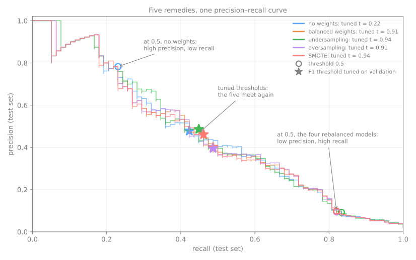
A lição: reamostragem e pesos basicamente movem o ponto de operação; mover o limiar faz o mesmo, de graça. Vale tentá-los, especialmente com modelos em que não é fácil trocar o limiar ou quando há pouquíssimos positivos, mas eles não são mágica e trazem duas armadilhas.
10. Duas armadilhas
Reamostrar antes da divisão
Etapa 4. Reamostrar o conjunto inteiro e depois dividir é o erro clássico, uma forma de vazamento de dados. A diferença entre as duas ordens está no que o "teste" passa a conter:
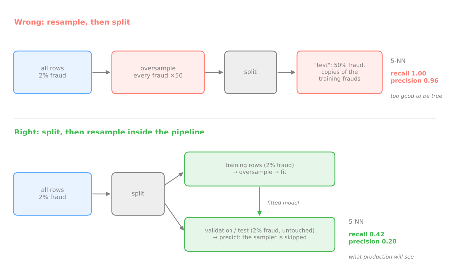
Medido com dois amostradores e dois modelos, contra a versão honesta (dividir primeiro, reamostrar só a parte de treino, dentro do pipeline):
from sklearn.neighbors import KNeighborsClassifier

X_dev, y_dev = np.r_[X_train, X_val], np.r_[y_train, y_val]      # tudo menos o conjunto de teste
for sampler in [RandomOverSampler(random_state=0), SMOTE(random_state=0)]:
    for clf in [KNeighborsClassifier(n_neighbors=5), LogisticRegression()]:
        # ERRADO: reamostrar o conjunto inteiro e depois dividir
        X_r, y_r = sampler.fit_resample(X, y)
        Xa, Xb, ya, yb = train_test_split(X_r, y_r, test_size=0.2, stratify=y_r, random_state=0)
        wrong = clf.fit(Xa, ya).predict(Xb)
        # CERTO: dividir primeiro, reamostrar só no ajuste
        right = make_imb_pipeline(sampler, clf).fit(X_dev, y_dev).predict(X_test)
        print(f"{type(sampler).__name__:17s} {type(clf).__name__:20s} "
              f"wrong: R {recall_score(yb, wrong):.2f} P {precision_score(yb, wrong):.2f}   "
              f"right: R {recall_score(y_test, right):.2f} P {precision_score(y_test, right):.2f}")
print(f"fraud share in the 'wrong' test set: {yb.mean():.0%}")
RandomOverSampler KNeighborsClassifier wrong: R 1.00 P 0.96   right: R 0.42 P 0.20
RandomOverSampler LogisticRegression   wrong: R 0.82 P 0.84   right: R 0.82 P 0.09
SMOTE             KNeighborsClassifier wrong: R 1.00 P 0.92   right: R 0.56 P 0.12
SMOTE             LogisticRegression   wrong: R 0.84 P 0.84   right: R 0.82 P 0.10
fraud share in the 'wrong' test set: 50%
Duas coisas dão errado ao mesmo tempo:
- o conjunto de teste está contaminado. Depois da sobreamostragem, cada fraude existe cerca de 50 vezes, então quase toda fraude da parte de "teste" tem cópias idênticas na parte de "treino". O k-NN as encontra e copia seu rótulo: recall 1,00 e precisão 0,96, contra 0,42 e 0,20 na versão honesta. O SMOTE mal melhora, já que cada ponto sintético de teste está num segmento entre pontos de treino;
- o conjunto de teste não tem mais a prevalência real. Ele tem 50% de fraudes em vez de 2%. Mesmo a regressão logística, que não consegue decorar cópias e mantém seu recall de 0,82, salta de precisão 0,09 para 0,84, um número que não diz nada sobre a produção, onde 98% das transações são legítimas.
Probabilidades distorcidas
Pesos ou reamostragem dizem ao modelo que as fraudes são 50% do mundo. Ele acredita:
p_smote = models['SMOTE'].predict_proba(X_test)[:, 1]
print(f"true fraud rate (test):       {y_test.mean():.4f}")
print(f"mean probability, no weights: {p_plain.mean():.4f}")
print(f"mean probability, balanced:   {p_w.mean():.4f}")
print(f"mean probability, SMOTE:      {p_smote.mean():.4f}")
odds = p_w / (1 - p_w) * n_c[1] / n_c[0]         # desfaz a reponderação: chances vezes n1/n0
print(f"balanced, corrected:          {(odds / (1 + odds)).mean():.4f}")
true fraud rate (test):       0.0195
mean probability, no weights: 0.0206
mean probability, balanced:   0.2370
mean probability, SMOTE:      0.2227
balanced, corrected:          0.0208
As probabilidades do modelo sem pesos têm média 0,0206, perto da taxa real de fraude, 0,0195. Os modelos com pesos balanceados e com SMOTE têm médias 0,237 e 0,223: mais de dez vezes altas demais. Se você só precisa de uma ordenação ou de uma decisão sim/não num limiar ajustado, isso não importa. Se precisa do número em si (uma perda esperada, um escore de risco mostrado a um médico, a fórmula de custo \(t^* = c_{FP}/(c_{FP}+c_{FN})\) da seção 6), importa. Para a regressão logística a correção é direta: multiplique as chances por \(n_1/n_0\) para desfazer os pesos, o que traz a média de volta a 0,0208 (Elkan, 2001). Para outros modelos, recalibre as probabilidades em dados separados; o CalibratedClassifierCV do scikit-learn faz isso, usando a validação cruzada que vem mais adiante no curso.
11. Uma ordem sensata de ataque
- Meça a coisa certa. Estratifique toda divisão. Reporte recall, precisão, curva PR e AP ao lado da prevalência, além da ROC AUC para a ordenação. A acurácia não diz quase nada aqui. Muitos "problemas de desbalanceamento" são problemas de métrica.
- Escolha o limiar em dados de validação, com o critério que a aplicação implica (uma meta de recall, uma razão de custos, o melhor F1 se nada mais for conhecido).
- Pesos de classe estão a um argumento de distância e não mudam os dados. Eles basicamente deslocam o ponto de operação; combinados com o passo 2, raramente mudam muito numa regressão logística, mas podem ajudar modelos cujo treino é dominado pela maioria (árvores, SVMs).
- Reamostragem só dentro de um pipeline do
imblearn, só nos dados de treino e comparada com os passos 2–3 no mesmo conjunto de validação. Espere diferenças pequenas. - Mais exemplos da minoria é o único remédio que melhora a própria ordenação. Nenhuma reamostragem inventa informação que os dados não têm.
Lab avançado — remédios, limiar e o único teste
Os passos 6 a 11 continuam a mesma triagem de mamografias, agora com a meta declarada no começo do lab fundamental: recall de pelo menos 0,80 nos casos malignos, com a melhor precisão possível.
Como fazer este lab em aula (cerca de 35 min, em duplas)
- Use o mesmo notebook do Colab do lab fundamental e vá até o passo 6. Nada para baixar.
- Os passos 6 a 11 usam os dados e o modelo dos passos 1 a 4. Se a sessão do Colab for nova (ou tiver expirado), clique na célula do passo 6 e use Ambiente de execução → Executar anteriores (Ctrl+F8) antes de continuar.
- O passo 7 usa o
imbalanced-learn. Ele já vem no Colab; se faltar, rode!pip install -q imbalanced-learnnuma célula antes. - A dinâmica é a mesma: Preveja antes de rodar, compare com a página e tente as Simulações antes de abrir a solução.
- Ritmo sugerido: passos 6 e 7 com a simulação em 15 min; passo 8 e a simulação em 10 min; passos 9 a 11 em 10 min.
Passo 6 — pesos de classe
Preveja. Com class_weight='balanced', o que você espera que mude mais: a ROC AUC (a ordenação) ou o número de regiões sinalizadas em 0,5?
lr_w = make_pipeline(StandardScaler(), LogisticRegression(class_weight='balanced')).fit(X_train, y_train)
p_val_w = lr_w.predict_proba(X_val)[:, 1]
pred = (p_val_w >= 0.5).astype(int)
print(f"flagged {pred.sum()}   recall {recall_score(y_val, pred):.3f}   precision {precision_score(y_val, pred):.3f}")
print(f"ROC AUC {roc_auc_score(y_val, p_val_w):.3f}   AP {average_precision_score(y_val, p_val_w):.3f}")
n0, n1 = np.bincount(y_train)
print(f"intercept shift {lr_w[-1].intercept_[0] - lr[-1].intercept_[0]:.2f}   log(n0/n1) = {np.log(n0 / n1):.2f}")
flagged 298   recall 0.904   precision 0.158
ROC AUC 0.954   AP 0.641
intercept shift 4.04   log(n0/n1) = 3.74
Como na aula, os pesos basicamente movem o ponto de operação: em 0,5 o modelo com pesos sinaliza 298 regiões em vez de 30, o recall salta de 0,442 para 0,904 e a precisão cai de 0,767 para 0,158. O intercepto sobe 4,04, perto de \(\log(n_0/n_1) = 3{,}74\). Em dados reais, a coincidência é mais frouxa do que na triagem de fraude simulada; a ordenação também se move um pouco: a ROC AUC sobe (0,946 → 0,954) enquanto a AP desce (0,653 → 0,641). As duas métricas pesam partes diferentes da curva; aqui, as mudanças estão dentro do ruído de 52 positivos.
Simulação: o limiar que imita os pesos. Se os pesos basicamente deslocam o ponto de operação, dá para chegar perto sem retreinar: corte os escores do modelo simples na prevalência do treino em vez de em 0,5. Compare esse ponto com o do modelo com pesos em 0,5 e conte em quantas regiões as duas regras discordam.
Solução
t_prev = y_train.mean()
a = p_val >= t_prev                               # modelo simples, limiar = prevalência do treino
b = p_val_w >= 0.5                                # modelo com pesos, limiar padrão
for name, f in [(f'simples, t = {t_prev:.4f}', a), ('balanced, t = 0.5   ', b)]:
    print(f"{name}: sinalizadas {f.sum():3d}  recall {recall_score(y_val, f):.3f}"
          f"  precisão {precision_score(y_val, f):.3f}")
print(f"regiões classificadas de forma diferente: {(a != b).sum()} de {len(y_val)}")
simples, t = 0.0233: sinalizadas 366  recall 0.923  precisão 0.131
balanced, t = 0.5   : sinalizadas 298  recall 0.904  precisão 0.158
regiões classificadas de forma diferente: 110 de 2237
Os dois pontos de operação são parecidos — recall alto, precisão por volta de 0,14 — e nenhum modelo precisou ser retreinado para chegar ao primeiro. Mas a correspondência é mais frouxa do que na triagem de fraude simulada da seção 9, em que as duas regras discordavam em 42 de 4.000 linhas: aqui são 110 de 2.237. O motivo é que pesar a classe não desloca exatamente o intercepto em dados reais; o passo 6 já tinha mostrado isso (4,04 contra \(\log(n_0/n_1) = 3{,}74\)). A lição prática continua: antes de retreinar com pesos, teste o que um limiar diferente faria, porque ele é de graça e reversível.
Passo 7 — reamostragem dentro de um pipeline do imblearn
Preveja. A subamostragem vai treinar em quantas linhas, mais ou menos? E o SMOTE? Qual das duas joga informação fora?
from imblearn.over_sampling import SMOTE
from imblearn.pipeline import make_pipeline as make_imb_pipeline
from imblearn.under_sampling import RandomUnderSampler

models = {
    'logistic': lr,
    'logistic, balanced': lr_w,
    'undersampling': make_imb_pipeline(StandardScaler(), RandomUnderSampler(random_state=0),
                                       LogisticRegression()),
    'SMOTE': make_imb_pipeline(StandardScaler(), SMOTE(random_state=0), LogisticRegression()),
}
for name in ['undersampling', 'SMOTE']:
    models[name].fit(X_train, y_train)            # o amostrador roda aqui, só no X_train
    X_r, y_r = models[name][1].fit_resample(X_train, y_train)
    print(f"{name:14s} trains on {len(y_r):5d} rows, {y_r.sum():4d} malignant")
Os dois amostradores vão em direções opostas. A subamostragem treina a regressão logística em 312 linhas (as 156 malignas mais 156 benignas sorteadas), descartando 6.397 regiões benignas. O SMOTE mantém todas as 6.553 regiões benignas e acrescenta 6.397 malignas sintéticas. Os dois vivem dentro de um pipeline do imblearn, então as linhas de validação e teste nunca são reamostradas: o predict_proba pula o amostrador. (A chamada a fit_resample aqui só conta as linhas; os pipelines já foram ajustados na linha anterior.)
Passo 8 — comparar no conjunto de validação
Preveja. Entre os quatro modelos, qual você espera que tenha a melhor ordenação (ROC AUC e AP)? A diferença vai ser grande?
from sklearn.metrics import f1_score

rows = []
for name, model in models.items():
    p = model.predict_proba(X_val)[:, 1]
    f = p >= 0.5
    rows.append({'model': name, 'ROC AUC': roc_auc_score(y_val, p), 'AP': average_precision_score(y_val, p),
                 'precision@0.5': precision_score(y_val, f), 'recall@0.5': recall_score(y_val, f),
                 'F1@0.5': f1_score(y_val, f)})
comparison = pd.DataFrame(rows).set_index('model')
print(comparison.round(3).to_string())
                    ROC AUC     AP  precision@0.5  recall@0.5  F1@0.5
model
logistic              0.946  0.653          0.767       0.442   0.561
logistic, balanced    0.954  0.641          0.158       0.904   0.269
undersampling         0.941  0.622          0.146       0.904   0.251
SMOTE                 0.955  0.647          0.164       0.885   0.276
O mesmo padrão da triagem de fraude simulada:
- ordenação: ROC AUC entre 0,941 e 0,955, AP entre 0,622 e 0,653. Com 52 positivos na validação, uma região maligna ordenada algumas posições acima ou abaixo move esses números mais ou menos nessa medida. Nenhum remédio é claramente melhor em ordenar; a subamostragem, que jogou fora 97% dos dados benignos, é ligeiramente a pior nas duas;
- em 0,5: o modelo simples está em precisão 0,767 / recall 0,442, os três rebalanceados em 0,146–0,164 / 0,885–0,904. Nenhum dos dois é o ponto de operação que queremos (recall ≥ 0,80 com a melhor precisão); ambos são só onde o 0,5 calha de cortar.
Como a escolha do limiar é nossa, a comparação justa é a da ordenação, que diz: fique com o modelo mais simples.
Simulação: comparar no limiar justo. A tabela acima corta os quatro modelos em 0,5, o que é injusto: cada um põe seus escores numa escala diferente. Refaça a comparação dando a cada modelo o seu próprio limiar, o que atinge recall ≥ 0,80 na validação com a melhor precisão. As diferenças aumentam ou diminuem?
Solução
print("modelo                limiar  recall  precisão  sinalizadas")
for name, model in models.items():
    p = model.predict_proba(X_val)[:, 1]
    prec, rec, thr = precision_recall_curve(y_val, p)
    ok = rec[:-1] >= 0.80
    i = int(np.argmax(np.where(ok, prec[:-1], -1)))
    print(f"{name:20s}{thr[i]:8.4f}{rec[i]:8.3f}{prec[i]:10.3f}{(p >= thr[i]).sum():13d}")
modelo                limiar  recall  precisão  sinalizadas
logistic              0.0632   0.808     0.294          143
logistic, balanced    0.6026   0.808     0.211          199
undersampling         0.6433   0.808     0.206          204
SMOTE                 0.6379   0.808     0.255          165
Com todos no mesmo recall, o que sobra para comparar é a precisão — e aí a regressão logística simples fica na frente (0,294 contra 0,206 a 0,255), ou seja, 143 regiões sinalizadas em vez de até 204 para encontrar os mesmos 42 cânceres. Repare nos limiares: 0,06 para o modelo simples e 0,60 a 0,64 para os rebalanceados. O mesmo ponto de operação aparece com números completamente diferentes no mostrador, o que é exatamente por que comparar modelos num limiar fixo de 0,5 não quer dizer nada. Nenhum remédio ganhou da ordenação original; o mais simples venceu.
Passo 9 — escolher o modelo e o limiar na validação
Preveja. Dado o que o passo 8 mostrou, qual modelo deve ser escolhido? E o limiar que atinge recall 0,80 vai ficar perto de 0,5 ou bem abaixo?
best_name = comparison['AP'].idxmax()
best = models[best_name]
p_val_best = best.predict_proba(X_val)[:, 1]
prec, rec, thr = precision_recall_curve(y_val, p_val_best)
ok = rec[:-1] >= 0.80                            # limiares que atingem a meta de recall
i = np.argmax(np.where(ok, prec[:-1], -1))       # entre eles, a melhor precisão
threshold = thr[i]
print(f"model: {best_name}   threshold {threshold:.4f}")
print(f"validation: recall {rec[i]:.3f}   precision {prec[i]:.3f}   flagged {(p_val_best >= threshold).sum()}")
O modelo com a melhor AP na validação é a regressão logística simples (0,653, à frente dos 0,647 do SMOTE por um fio). Entre os seus limiares que chegam a recall 0,80 na validação, o de melhor precisão é 0,0632: o modelo sinaliza toda região com probabilidade estimada de malignidade acima de 6,3%. Na validação isso significa 143 regiões sinalizadas, 42 dos 52 cânceres encontrados (0,808), precisão 0,294. Um limiar de 0,06 pode parecer estranho, mas é a aritmética de uma taxa base de 2,3% e de uma perda que custa muito mais do que uma segunda olhada.
Passo 10 — o único teste
Preveja. O recall no teste vai ficar acima ou abaixo dos 0,808 da validação? Com 52 casos malignos, quanto vale um caso?
from sklearn.metrics import confusion_matrix

p_test = best.predict_proba(X_test)[:, 1]
pred_test = (p_test >= threshold).astype(int)
print(confusion_matrix(y_test, pred_test, labels=[1, 0]))
print(f"recall {recall_score(y_test, pred_test):.3f}   precision {precision_score(y_test, pred_test):.3f}"
      f"   flagged {pred_test.sum()} of {len(pred_test)}")
print(f"ROC AUC {roc_auc_score(y_test, p_test):.3f}   AP {average_precision_score(y_test, p_test):.3f}")
Uma vez, no fim, o modelo e o limiar escolhidos encontram o conjunto de teste. 43 das 52 regiões malignas são encontradas (recall 0,827) e 9 passam; 97 regiões benignas são sinalizadas, então o radiologista revisa 140 de 2.237 regiões (6,3%) e cerca de 1 em cada 3 delas é um câncer (precisão 0,307). As estimativas da validação (recall 0,808, precisão 0,294) se sustentaram. Dois cuidados. Com 52 positivos, um câncer vale 1,9 ponto de recall, então "0,827" quer dizer "43, mais ou menos alguns"; a ROC AUC, 0,913 aqui contra 0,946 na validação, se move tanto quanto isso entre duas divisões deste tamanho. E se 0,827 decepcionar você, voltar agora para mudar o limiar transformaria o conjunto de teste num conjunto de validação.
Passo 11 — a escada grosseira de um k-NN
Preveja. Com \(k = 5\), quantas probabilidades distintas o k-NN pode produzir? Quantos pontos a curva ROC dele vai ter e isso é um problema para a nossa meta de recall 0,80?
from sklearn.neighbors import KNeighborsClassifier

knn = make_pipeline(StandardScaler(), KNeighborsClassifier(n_neighbors=5)).fit(X_train, y_train)
p_knn = knn.predict_proba(X_val)[:, 1]
print("distinct probabilities:", np.unique(p_knn))
fpr_k, tpr_k, thr_k = roc_curve(y_val, p_knn)
print(f"ROC points: {len(thr_k)}   ROC AUC {roc_auc_score(y_val, p_knn):.3f}   AP {average_precision_score(y_val, p_knn):.3f}")
for t, f, r in zip(thr_k, fpr_k, tpr_k):
    print(f"threshold {t:.1f}   FPR {f:.3f}   recall {r:.3f}")

fig, ax = plt.subplots(figsize=(5, 4))
RocCurveDisplay.from_predictions(y_val, p_val, ax=ax, name='logistic')
RocCurveDisplay.from_predictions(y_val, p_knn, ax=ax, name='5-NN')
plt.show()
distinct probabilities: [0.  0.2 0.4 0.6 0.8 1. ]
ROC points: 7   ROC AUC 0.935   AP 0.670
threshold inf   FPR 0.000   recall 0.000
threshold 1.0   FPR 0.001   recall 0.308
threshold 0.8   FPR 0.002   recall 0.481
threshold 0.6   FPR 0.004   recall 0.558
threshold 0.4   FPR 0.007   recall 0.750
threshold 0.2   FPR 0.038   recall 0.885
threshold 0.0   FPR 1.000   recall 1.000
Com \(k = 5\), a probabilidade de malignidade é a fração de regiões malignas entre os 5 vizinhos mais próximos, então só pode ser 0; 0,2; 0,4; 0,6; 0,8 ou 1: seis limiares, sete pontos ROC contando o canto. A ordenação não é ruim (ROC AUC 0,935, AP 0,670, perto da regressão logística), mas o cardápio de pontos de operação é curto. Para a nossa meta, recall ≥ 0,80, o k-NN precisa saltar de 0,750 (limiar 0,4) para 0,885 (limiar 0,2, FPR 0,038): não há nada no meio. O último segmento da curva ROC dele, de FPR 0,038 até 1, é uma reta: a AUC conta a área sob ela, mas o único jeito de operar sobre ela é sinalizar ao acaso as regiões com probabilidade 0. Um \(k\) maior dá mais valores distintos e uma curva mais fina.
Para fechar a aula. Em uma frase cada: (1) o que os pesos de classe mudaram e o que não mudaram? (2) Por que reamostrar antes de dividir inflaciona o resultado de duas maneiras? (3) Por que a regressão logística simples venceu a comparação?
Sua vez (avançado)
Para casa, com mais tempo:
- Um custo em vez de uma meta. Suponha que deixar passar um câncer custe 20 vezes uma nova convocação desnecessária. No conjunto de validação, calcule o custo \(20 \cdot FN + FP\) para cada limiar do modelo escolhido e encontre o mínimo. Compare com a fórmula \(t^* = 1/(1+20)\). Por que eles diferem?
- Reamostrar antes de dividir. Aplique
SMOTEa todo oX, y, depois divida 80/20 e ajuste um 5-NN. Compare seu recall e sua precisão com o passo 10. Quais duas coisas deram errado? - Mais vizinhos. Repita o passo 11 com \(k = 15\) e \(k = 51\). Quantas probabilidades distintas, quantos pontos ROC e o que acontece com a AUC? Quais pontos de operação perto de recall 0,80 passam a existir?
- A sorte da divisão. Troque
random_state=7no passo 2 por 0, 1, 2, 3 e 4 e rode de novo os passos 2–10. Quanto se movem o limiar escolhido e o recall de teste? O que isso diz sobre reportar "recall 0,827" com três casas decimais?
Referências
- Hanley, J. A.; McNeil, B. J. "The Meaning and Use of the Area under a Receiver Operating Characteristic (ROC) Curve." Radiology 143, no. 1 (1982): 29–36 — a AUC como a probabilidade de ordenar um positivo ao acaso acima de um negativo ao acaso. DOI
- Fawcett, T. "An Introduction to ROC Analysis." Pattern Recognition Letters 27, no. 8 (2006): 861–874. DOI
- Davis, J.; Goadrich, M. "The Relationship Between Precision-Recall and ROC Curves." Proceedings of the 23rd International Conference on Machine Learning (ICML) (2006): 233–240 — por que pontos PR não podem ser ligados por retas. DOI
- Saito, T.; Rehmsmeier, M. "The Precision-Recall Plot Is More Informative than the ROC Plot When Evaluating Binary Classifiers on Imbalanced Datasets." PLoS ONE 10, no. 3 (2015): e0118432. DOI
- Youden, W. J. "Index for Rating Diagnostic Tests." Cancer 3, no. 1 (1950): 32–35. DOI
- Elkan, C. "The Foundations of Cost-Sensitive Learning." Proceedings of the 17th International Joint Conference on Artificial Intelligence (IJCAI) (2001): 973–978 — o limiar ótimo para custos dados e como a reponderação muda as probabilidades. PDF
- Chawla, N. V.; Bowyer, K. W.; Hall, L. O.; Kegelmeyer, W. P. "SMOTE: Synthetic Minority Over-sampling Technique." Journal of Artificial Intelligence Research 16 (2002): 321–357. DOI
- He, H.; Garcia, E. A. "Learning from Imbalanced Data." IEEE Transactions on Knowledge and Data Engineering 21, no. 9 (2009): 1263–1284 — um panorama de métodos de amostragem, sensíveis a custo e de avaliação. DOI
- Lemaître, G.; Nogueira, F.; Aridas, C. K. "Imbalanced-learn: A Python Toolbox to Tackle the Curse of Imbalanced Datasets in Machine Learning." JMLR 18, no. 17 (2017): 1–5. PDF
- imbalanced-learn — reamostragem (SMOTE, sub/sobreamostragem) dentro de pipelines.
Quiz
O quiz cobre a abordagem fundamental.