Máquinas de Vetores de Suporte
A SVM (Cortes & Vapnik, 1995) coroou a era do aprendizado estatístico: um classificador derivado de um princípio geométrico elegante — maximizar a margem — com teoria rigorosa por trás e um truque que permite a um método linear traçar fronteiras extremamente não lineares. Antes do deep learning, as SVMs eram o estado da arte em quase toda parte; elas continuam excelentes em problemas de porte pequeno a médio e de alta dimensão.
Você já conhece os dois parentes mais próximos dela. Como a regressão logística, uma SVM linear calcula um escore \(f(x) = w^\top x + b\) e prevê pelo sinal dele; o C dela é a mesma força de regularização inversa que você ajustou na validação cruzada. Como o k-NN, uma SVM com kernel prevê a partir da semelhança de um ponto novo com pontos de treino guardados; o que muda é que só alguns deles (os vetores de suporte) votam, com pesos aprendidos. Todo número citado vem dos blocos de código ou dos scripts das figuras que ficam ao lado desta página.
Como esta aula está organizada
A aula tem duas abordagens. Cada uma tem slides, texto e um lab para fazer em aula no Colab; o quiz do fim cobre a fundamental. Comece pela fundamental: a avançada parte dela.
| Abordagem fundamental | Abordagem avançada | |
|---|---|---|
| pergunta | Entre infinitas retas que separam os dados, qual escolher — e por quê? | Como uma máquina linear traça fronteiras curvas e o que isso custa |
| conteúdo | margem máxima, distância a um hiperplano, vetores de suporte, margem suave, perda hinge, o botão \(C\) | o truque do kernel, RBF, \(C\) e \(\gamma\) juntos, escalonamento, escores e probabilidades, multiclasse, custo |
| lab em aula | radar: modelos lineares, passos 1 a 4 | ligar o kernel e ajustá-lo, passos 5 a 9 |
| ao final, você sabe | calcular a margem à mão; dizer quais pontos sustentam a solução; ler a perda hinge; prever o efeito do \(C\) | escolher um kernel; ajustar \(C\) e \(\gamma\) juntos; reconhecer subajuste e sobreajuste no mapa; saber quando a SVM deixa de ser prática |
Os dois labs usam o mesmo notebook no Colab: a parte fundamental vai do passo 1 ao 4; a avançada, do 5 ao 9. Tudo roda no navegador; não é preciso baixar nada.
Abordagem fundamental
Uma pergunta guia esta parte: quando infinitas retas separam os dados, qual delas escolher? A resposta da SVM é geométrica e leva a um problema de otimização com um único ótimo global, em que só alguns pontos de treino importam.
Esta parte segue um pipeline em três etapas, desenhado abaixo: 1. a rua mais larga, a margem como o critério que escolhe entre as retas separadoras; 2. geometria à mão, o problema de otimização e seus vetores de suporte; 3. margem suave e C, para classes que se sobrepõem. Cada etapa leva à sua seção e, nos slides, uma faixa embaixo mostra em que etapa você está.
- A rua mais largamuitas retas separam; a margem escolhe
- Geometria à mãomargem com sinal, o problema de otimização, vetores de suporte
- Margem suave e Cfolga, perda hinge, o que o C compra
Slides da abordagem fundamental
Clique nos slides e use as setas ← → para navegar; F abre em tela cheia e Esc mostra todos os slides. Abrir os slides numa aba nova
1. Muitas retas separam os dados — qual escolher?
Etapa 1. Na aula de regressão logística os rótulos eram \(y \in \{0, 1\}\). As SVMs usam \(y \in \{-1, +1\}\), o que torna central uma grandeza: a margem com sinal \(m = y \cdot f(x)\). Ela é positiva quando o ponto está do lado certo da fronteira \(f(x) = 0\) e grande quando está longe dela.
Quando duas classes podem ser separadas por uma reta, infinitas retas fazem isso. Todas têm 100% de acurácia no treino, então a acurácia não consegue escolher entre elas. A resposta da SVM é geométrica: escolha a reta que fica o mais longe possível do ponto mais próximo de cada classe — a "rua" mais larga entre as classes (script da figura):
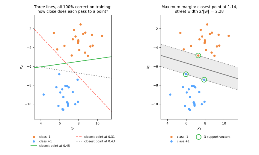
As três retas da esquerda são todas perfeitas no treino, mas cada uma passa a uma distância de apenas 0,31 a 0,45 de algum ponto: um ponto novo só um pouco diferente daquele pode cair do lado errado. A reta de margem máxima, à direita, mantém todo ponto de treino a pelo menos 1,14 de distância e a rua entre as linhas tracejadas tem 2,28 de largura. Os pontos circulados ficam exatamente nas bordas da rua. São os vetores de suporte: a solução depende deles e de nada mais.
2. A geometria, à mão
Distância a um hiperplano
Etapa 2. Para um hiperplano \(w^\top x + b = 0\), a distância de um ponto \(x\) até ele é
Multiplicar \(w\) e \(b\) pela mesma constante não move o hiperplano, então a SVM fixa a escala: os pontos mais próximos precisam ter \(\lvert w^\top x + b \rvert = 1\). Esses pontos ficam nas duas linhas tracejadas \(f(x) = +1\) e \(f(x) = -1\), cada uma a distância \(1/\lVert w \rVert\) da fronteira, então a rua tem largura \(2 / \lVert w \rVert\). Maximizar a rua é o mesmo que minimizar \(\lVert w \rVert\):
É um programa quadrático convexo: um único ótimo global, sem inicialização aleatória, sem taxa de aprendizado.
Ensaio numérico: seis pontos
Tome três pontos de cada classe:
| ponto | \(x_1\) | \(x_2\) | \(y\) |
|---|---|---|---|
| A | 0 | 0 | −1 |
| B | 1 | 0 | −1 |
| C | 0 | 1 | −1 |
| D | 2 | 2 | +1 |
| E | 3 | 2 | +1 |
| F | 2 | 3 | +1 |
À mão. Os dois grupos se encaram ao longo da diagonal, então, por simetria, a melhor fronteira é perpendicular a ela: \(w = (a, a)\), uma reta \(x_1 + x_2 = \text{const}\). Os negativos mais próximos são B e C (\(x_1 + x_2 = 1\)); o positivo mais próximo é D (\(x_1 + x_2 = 4\)). A fronteira fica no meio, em \(x_1 + x_2 = 2{,}5\). A condição de escala diz \(f = +1\) em D e \(f = -1\) em B:
Logo \(w = (0{,}667;\ 0{,}667)\), \(\lVert w \rVert = \tfrac{2}{3}\sqrt{2} = 0{,}943\) e a rua tem \(2 / 0{,}943 = 2{,}121\) de largura — exatamente a distância entre as retas \(x_1 + x_2 = 1\) e \(x_1 + x_2 = 4\), que é \(3/\sqrt2\).
A biblioteca confirma. Uma margem rígida (nenhuma violação permitida) é SVC(kernel='linear') com um C enorme; o porquê do C fica claro na próxima seção:
import numpy as np
import pandas as pd
from sklearn.svm import SVC

X = np.array([[0, 0], [1, 0], [0, 1], [2, 2], [3, 2], [2, 3]])
y = np.array([-1, -1, -1, 1, 1, 1])

svm = SVC(kernel='linear', C=1e6, tol=1e-8).fit(X, y)     # C enorme = margem rígida
w, b = svm.coef_[0], svm.intercept_[0]
print("w =", w.round(3), "  b =", round(b, 3))
print("support vectors:", svm.support_, "->", X[svm.support_].tolist())
print(f"street width 2/||w|| = {2 / np.linalg.norm(w):.3f}")
w = [0.667 0.667]   b = -1.667
support vectors: [1 2 3] -> [[1, 0], [0, 1], [2, 2]]
street width 2/||w|| = 2.121
Mesmo \(w\), mesmo \(b\), mesma largura; os vetores de suporte são as linhas 1, 2 e 3: B, C e D, os três pontos nas bordas da rua. O escore e a distância de cada ponto:
f = X @ w + b                                  # o mesmo que svm.decision_function(X)
print(pd.DataFrame({'point': list('ABCDEF'), 'y': y, 'f(x)': f.round(3),
                    'm = y·f(x)': (y * f).round(3),
                    'distance': (np.abs(f) / np.linalg.norm(w)).round(3)}).to_string(index=False))
point  y   f(x)  m = y·f(x)  distance
    A -1 -1.667       1.667     1.768
    B -1 -1.000       1.000     1.061
    C -1 -1.000       1.000     1.061
    D  1  1.000       1.000     1.061
    E  1  1.667       1.667     1.768
    F  1  1.667       1.667     1.768
Os vetores de suporte têm \(m = 1\) exatamente e ficam a distância \(1{,}061\), meia rua. A, E e F têm \(m > 1\): estão mais longe do que precisariam e a solução os ignora.
Só os vetores de suporte importam
O solver na verdade trabalha num problema diferente, mas equivalente (o dual), com um peso \(\alpha_i \geq 0\) por ponto de treino. Depois, reconstrói \(w\) a partir deles:
Pontos além da margem terminam com \(\alpha_i = 0\). O scikit-learn guarda os produtos não nulos \(\alpha_i y_i\) em dual_coef_:
print("alpha_i * y_i of the support vectors:", svm.dual_coef_.round(3))
print("w rebuilt from them:", (svm.dual_coef_ @ svm.support_vectors_).round(3))
\(w = -\tfrac{2}{9}(1, 0) - \tfrac{2}{9}(0, 1) + \tfrac{4}{9}(2, 2) = (\tfrac{2}{3}, \tfrac{2}{3})\). Três pontos de seis carregam o modelo inteiro. A consequência prática: apagar um ponto que não é vetor de suporte não muda nada; apagar um vetor de suporte muda a resposta.
for drop, label in [(4, 'E = (3, 2), not a support vector'), (3, 'D = (2, 2), a support vector')]:
    keep = np.arange(len(X)) != drop
    s = SVC(kernel='linear', C=1e6, tol=1e-8).fit(X[keep], y[keep])
    print(f"without {label}: w = {s.coef_[0].round(3)}, b = {s.intercept_[0]:.3f}, "
          f"width {2 / np.linalg.norm(s.coef_):.3f}")
without E = (3, 2), not a support vector: w = [0.667 0.667], b = -1.667, width 2.121
without D = (2, 2), a support vector: w = [0.5 0.5], b = -1.500, width 2.828
Sem D, os positivos mais próximos passam a ser E e F (\(x_1 + x_2 = 5\)), a rua se alarga para \(4/\sqrt2 = 2{,}828\) e a fronteira vai para \(x_1 + x_2 = 3\). A regressão logística se comporta de outro jeito: todo ponto de treino tem peso não nulo na solução, então remover qualquer ponto move um pouco a fronteira.
3. Margem suave e C
Folga e a perda hinge
Etapa 3. Classes reais se sobrepõem; nesse caso, nenhuma rua fica vazia. A margem suave deixa o ponto \(i\) violar a margem por uma folga \(\xi_i \geq 0\) e cobra por isso:
A folga mais barata é \(\xi_i = \max(0,\, 1 - m_i)\), com \(m_i = y_i f(x_i)\). Essa função tem nome — perda hinge (dobradiça) — e substituí-la mostra a SVM como "perda + penalidade":
Compare com o que a LogisticRegression do scikit-learn minimiza (penalidade L2):
Mesma forma, mesmo \(C\) no mesmo lugar: um \(C\) grande torna os erros caros em relação a \(\lVert w \rVert\) (regularização fraca), um \(C\) pequeno os torna baratos (regularização forte). É a mesma regularização inversa que você ajustou para a regressão logística na validação cruzada e a mesma forma "perda + penalidade" do Ridge. A única diferença entre os dois classificadores é a perda.
Ensaio numérico: quatro pontos contra a solução dos seis
Mantenha \(w = (0{,}667;\ 0{,}667)\), \(b = -1{,}667\) do exemplo à mão e calcule o escore de quatro pontos novos da classe \(+1\):
pts = np.array([[3, 3], [2, 2], [1.5, 1.5], [1, 0.5]])
m = +1 * (pts @ w + b)                                     # y = +1 para os quatro
print(pd.DataFrame({'point': ['(3, 3)', '(2, 2)', '(1.5, 1.5)', '(1, 0.5)'],
                    'm = y·f(x)': m.round(3),
                    'hinge': np.maximum(0, 1 - m).round(3),
                    'log loss': np.log1p(np.exp(-m)).round(3),
                    '0-1 loss': (m <= 0).astype(int)}).to_string(index=False))
     point  m = y·f(x)  hinge  log loss  0-1 loss
    (3, 3)       2.333  0.000     0.093         0
    (2, 2)       1.000  0.000     0.313         0
(1.5, 1.5)       0.333  0.667     0.540         0
  (1, 0.5)      -0.667  1.667     1.081         1
Confira a primeira e a terceira linhas com uma calculadora: \(f(3,3) = \tfrac{2}{3} \cdot 6 - \tfrac{5}{3} = \tfrac{7}{3} = 2{,}333\), hinge \(\max(0;\ 1 - 2{,}333) = 0\); \(f(1{,}5;\ 1{,}5) = \tfrac{2}{3} \cdot 3 - \tfrac{5}{3} = \tfrac{1}{3}\), hinge \(1 - 0{,}333 = 0{,}667\). Quatro situações:
- (3, 3), bem além da margem: hinge 0. A log loss é pequena (0,093), mas não zero, então a regressão logística ainda "escuta" esse ponto;
- (2, 2), exatamente sobre a margem: hinge ainda 0;
- (1,5; 1,5), lado certo, mas dentro da rua: hinge 0,667, embora a perda 0-1 diga "certo";
- (1; 0,5), lado errado: hinge 1,667, crescendo linearmente com a distância.
A figura mostra as três perdas como funções de \(m\), com os quatro pontos marcados (script da figura):
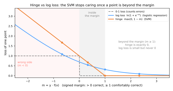
As duas perdas são convexas; é por isso que ambas podem ser otimizadas com confiança. A hinge é, além disso, uma cota superior da perda 0-1: nunca cobra menos que a contagem de erros. A log loss, escrita aqui com o logaritmo natural, não chega a ser: do lado errado e perto da fronteira (\(-0{,}54 < m \leq 0\)) ela custa menos que 1, como mostra a figura; em base 2, \(\log_2(1 + e^{-m})\), seria. A parte plana da hinge é de onde vem a esparsidade da SVM: pontos com \(m > 1\) não contribuem nada para a perda e recebem \(\alpha_i = 0\).
O que o C faz, medido
Em 100 pontos de duas nuvens que se sobrepõem, ajuste uma SVM linear para vários valores de \(C\):
from sklearn.datasets import make_blobs
from sklearn.model_selection import StratifiedKFold, cross_val_score

X, y = make_blobs(n_samples=100, centers=2, cluster_std=1.6, random_state=7)
cv = StratifiedKFold(n_splits=5, shuffle=True, random_state=0)
for C in [0.001, 0.01, 0.1, 1, 100]:
    svm = SVC(kernel='linear', C=C).fit(X, y)
    width = 2 / np.linalg.norm(svm.coef_)
    acc = cross_val_score(SVC(kernel='linear', C=C), X, y, cv=cv).mean()
    print(f"C = {C:<6g} width {width:5.2f} · support vectors {svm.n_support_.sum():3d} · "
          f"train {svm.score(X, y):.2f} · CV {acc:.3f}")
C = 0.001  width  9.23 · support vectors  78 · train 0.99 · CV 1.000
C = 0.01   width  5.13 · support vectors  27 · train 1.00 · CV 0.990
C = 0.1    width  2.63 · support vectors  12 · train 1.00 · CV 1.000
C = 1      width  1.33 · support vectors   6 · train 1.00 · CV 0.990
C = 100    width  0.39 · support vectors   3 · train 1.00 · CV 0.990
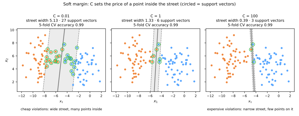
Leia a tabela de cima para baixo:
- \(C\) pequeno: violações são baratas, então o otimizador prefere um \(\lVert w \rVert\) pequeno, isto é, uma rua larga. Muitos pontos caem dentro dela e todos eles são vetores de suporte (78 de 100 com \(C = 0{,}001\));
- \(C\) grande: violações são caras. A rua encolhe até quase nenhum ponto ficar dentro dela: com \(C = 100\) ela tem 0,39 de largura e depende de 3 pontos. A margem rígida é o limite \(C \to \infty\); é por isso que o exemplo à mão usou \(C = 10^6\).
O número de vetores de suporte é uma leitura direta de quão regularizado está o modelo. Neste problema fácil a acurácia em validação cruzada quase não se move (0,99–1,00): a geometria muda muito e o escore não; em dados mais difíceis, como você verá com kernels, o \(C\) errado custa acurácia de verdade. O \(C\) é um hiperparâmetro, escolhido com validação cruzada, como o C da regressão logística.
Experimente. O simulador resolve o problema de margem suave ao vivo; mexa no \(C\) e arraste os pontos:
Ideia-chave
A SVM é "perda + penalidade" como o Ridge, com a perda hinge no lugar da log loss. A parte plana da hinge — custo exatamente zero para \(m > 1\) — é de onde vem a esparsidade: pontos bem classificados recebem \(\alpha_i = 0\) e somem da solução.
4. Resumo: a SVM linear em cinco linhas
- A margem é a régua. Entre todas as retas que separam, escolha a que fica mais longe do ponto mais próximo: a rua de largura \(2 / \lVert w \rVert\).
- Maximizar a rua = minimizar \(\lVert w \rVert\), sujeito a \(y_i f(x_i) \geq 1\). É um problema quadrático convexo: um ótimo global, sem taxa de aprendizado.
- Só os vetores de suporte importam. \(w = \sum_i \alpha_i y_i x_i\) e \(\alpha_i = 0\) para todo ponto além da margem.
- A margem suave cobra \(C\) por unidade de violação; a folga mais barata é a perda hinge \(\max(0, 1 - m)\).
- O \(C\) é o mesmo da regressão logística: pequeno = regularização forte = rua larga = muitos vetores de suporte.
| sintoma | o que está acontecendo | o que fazer |
|---|---|---|
| quase todos os pontos são vetores de suporte | \(C\) muito pequeno: a rua engoliu os dados | aumentar o \(C\) |
| 2 ou 3 vetores de suporte e acurácia de treino 1,00 | \(C\) muito grande: margem quase rígida | diminuir o \(C\); olhar a CV, não o treino |
| escores enormes ou minúsculos | atributos em escalas diferentes | StandardScaler dentro do pipeline |
| a fronteira linear não serve | o problema não é linearmente separável | o kernel, na parte avançada |
Lab fundamental — a SVM linear
O problema. O conjunto Ionosphere (Sigillito et al., 1989) vem de um arranjo de radar em Goose Bay, no Labrador, que envia pulsos à ionosfera. Cada uma das 351 linhas é um retorno, descrito por 34 números (17 medições de pulso, cada uma um par de valores da função de autocorrelação complexa). Um retorno "bom" (g) mostra indícios de estrutura na ionosfera; um "ruim" (b) atravessa a ionosfera. A tarefa: classificar os retornos automaticamente. É um problema pequeno, de alta dimensão e com fronteira não linear, o tipo de problema em que kernels fazem diferença.
O fluxo é o da aula de validação: trancar um conjunto de teste, comparar modelos nos mesmos folds de validação cruzada e tocar o teste uma única vez, no passo 9.
Como fazer este lab em aula (cerca de 30 min, em duplas)
- Abra o notebook do lab no Colab. Não é preciso baixar nem instalar nada: o Colab roda no navegador. Para guardar as suas respostas, salve uma cópia no seu Drive (Arquivo → Salvar uma cópia no Drive) antes de editar. Rode as células em ordem, numa mesma sessão.
- Este lab corresponde aos passos 1 a 4 do notebook. O lab avançado continua no mesmo notebook, a partir do passo 5.
- Cada passo começa com um Preveja: responda com a dupla antes de rodar a célula. Errar a previsão é o que torna o resultado memorável.
- Depois de rodar, compare com a saída e a leitura desta página. Toda saída aqui é exatamente o que o código imprime.
- As Simulações pedem que vocês escrevam um pequeno experimento em Python: mudar uma entrada e observar o que acontece com a saída. Nada de conta à mão. A solução fica recolhida logo abaixo: tente antes de abrir.
- Ritmo sugerido: passos 1 a 3 em 10 min; passo 4 e as duas simulações em 20 min.
Passo 1 — carregar e olhar
Preveja. Antes de rodar: para uma SVM, o que importa mais saber sobre as 34 colunas — a média delas, a faixa de valores ou quantas são categóricas? Por quê?
import numpy as np
import pandas as pd
from sklearn.datasets import fetch_openml

data = fetch_openml(data_id=59, as_frame=True)       # Ionosphere (UCI)
X = data.data                                        # 34 atributos numéricos
y = (data.target == 'g').astype(int)                 # 1 = retorno de radar "bom", 0 = "ruim"
print(X.shape)
print(y.value_counts())
print(f"values from {X.min().min():.0f} to {X.max().max():.0f} · "
      f"constant columns: {list(X.columns[X.std() == 0])}")
(351, 34)
class
1    225
0    126
Name: count, dtype: int64
values from -1 to 1 · constant columns: ['a02']
351 retornos: 225 bons (64,1%) e 126 ruins. Dois detalhes importam para uma SVM. Primeiro, todo valor já está entre −1 e 1 (os atributos são valores de autocorrelação normalizados; a01 é um indicador 0/1), então as escalas já são comparáveis antes de qualquer pré-processamento; mesmo assim padronizamos dentro do pipeline, o que não custa nada e deixa todo atributo com variância 1. Segundo, a coluna a02 é zero em todas as linhas. Ela não carrega informação e é inofensiva: o StandardScaler deixa uma coluna constante em 0, então ela não soma nada a nenhuma distância ou kernel.
Passo 2 — trancar o conjunto de teste
Preveja. Com 88 linhas de teste, quanto vale uma única linha em pontos de acurácia? Isso muda o quanto você deve confiar na terceira casa decimal do número final?
from sklearn.model_selection import train_test_split

X_train, X_test, y_train, y_test = train_test_split(
    X, y, test_size=0.25, stratify=y, random_state=42)
print(X_train.shape, X_test.shape)
print(f"share of 'good': train {y_train.mean():.3f} · test {y_test.mean():.3f}")
263 linhas para desenvolvimento e 88 trancadas até o passo 9, ambas com a mesma fração de 64% de retornos bons graças ao stratify=y. Com 88 linhas de teste, uma única linha vale 1,14 ponto de acurácia; lembre-se disso ao ler o número final.
Passo 3 — um baseline e os folds que todos compartilham
Preveja. Responder sempre "bom" acerta quantos por cento? E qual vai ser a ROC AUC desse baseline?
from sklearn.dummy import DummyClassifier
from sklearn.model_selection import StratifiedKFold, cross_validate

cv = StratifiedKFold(n_splits=5, shuffle=True, random_state=42)


def cv_summary(model):
    r = cross_validate(model, X_train, y_train, cv=cv, scoring=['accuracy', 'roc_auc'])
    return {metric: f"{r['test_' + metric].mean():.3f} ± {r['test_' + metric].std():.3f}"
            for metric in ['accuracy', 'roc_auc']}


print(cv_summary(DummyClassifier(strategy='most_frequent')))
Responder sempre "bom" acerta 64,3% das vezes e a ROC AUC é 0,5 porque ele não ordena nada. Toda acurácia deve ser lida contra 0,643, não contra 0,5. O objeto cv é criado uma vez e reutilizado em todos os passos seguintes, então todos os modelos são avaliados nos mesmos cinco folds; as diferenças entre eles vêm dos modelos, não da sorte da divisão. A cv_summary reporta a média ± desvio-padrão nos cinco folds.
Passo 4 — três modelos que você conhece, nos mesmos folds
Preveja. A regressão logística e a SVM linear traçam ambas um hiperplano nos mesmos 34 atributos padronizados e só discordam na perda. Você espera uma diferença grande entre elas ou menor que o desvio entre folds?
from sklearn.linear_model import LogisticRegression
from sklearn.neighbors import KNeighborsClassifier
from sklearn.pipeline import make_pipeline
from sklearn.preprocessing import StandardScaler
from sklearn.svm import SVC

models = {
    'logistic regression': make_pipeline(StandardScaler(), LogisticRegression(max_iter=1000)),
    'k-NN (k = 5)': make_pipeline(StandardScaler(), KNeighborsClassifier()),
    'linear SVM (C = 1)': make_pipeline(StandardScaler(), SVC(kernel='linear')),
}
print(pd.DataFrame({name: cv_summary(m) for name, m in models.items()}).T)
                          accuracy        roc_auc
logistic regression  0.882 ± 0.021  0.895 ± 0.044
k-NN (k = 5)         0.818 ± 0.025  0.901 ± 0.031
linear SVM (C = 1)   0.886 ± 0.017  0.850 ± 0.052
Como ler:
- Regressão logística e SVM linear empatam na acurácia (0,882 contra 0,886, uma diferença muito menor que qualquer um dos desvios-padrão). As duas traçam um hiperplano nos mesmos 34 atributos padronizados; só discordam na perda, o que aqui quase não importa.
- A ROC AUC da SVM linear é menor (0,850 ± 0,052 contra 0,895 ± 0,044), mas a diferença é de cerca de um desvio-padrão entre folds: sugestiva, não conclusiva.
- O k-NN tem a pior acurácia (0,818) e a melhor ROC AUC dos três (0,901). A ordenação que ele faz dos retornos é boa; a decisão padrão (maioria de 5 vizinhos), não. Um modelo local vê algo que os dois lineares perdem, o que é uma pista de que a fronteira não é um hiperplano.
Simulação: só os vetores de suporte importam. A seção 2 afirmou que apagar um ponto que não é vetor de suporte não muda nada. Teste isso nos dados do lab: padronize uma vez (para isolar o efeito, já que um scaler reajustado mudaria tudo), ajuste uma SVM linear, descubra quais linhas são vetores de suporte e refaça o ajuste sem uma linha de cada tipo. O que acontece com \(\lVert w \rVert\)?
Solução
Z = StandardScaler().fit_transform(X_train)   # padroniza UMA vez, para isolar o efeito
lin = SVC(kernel='linear').fit(Z, y_train)
sv = set(lin.support_)
print(f"{len(sv)} vetores de suporte de {len(Z)} linhas")

for label, drop in [('uma linha que não é VS', next(i for i in range(len(Z)) if i not in sv)),
                    ('um vetor de suporte', lin.support_[0])]:
    keep = np.arange(len(Z)) != drop
    s = SVC(kernel='linear').fit(Z[keep], y_train.iloc[keep])
    print(f"sem {label:22s}: ||w|| {np.linalg.norm(s.coef_):.6f} "
          f"(era {np.linalg.norm(lin.coef_):.6f}) · vetores de suporte {s.n_support_.sum()}")
70 vetores de suporte de 263 linhas
sem uma linha que não é VS: ||w|| 3.808782 (era 3.808803) · vetores de suporte 70
sem um vetor de suporte   : ||w|| 3.767861 (era 3.808803) · vetores de suporte 70
Apagar uma das 193 linhas que não são vetores de suporte deixa \(\lVert w \rVert\) praticamente igual: a diferença, 0,00002, é a tolerância do solver, não um modelo diferente. Apagar um vetor de suporte já muda a segunda casa decimal (3,7679 contra 3,8088), uma diferença cerca de duas mil vezes maior. A solução depende de 70 pontos de 263 e é literalmente indiferente aos outros 193 — o que a regressão logística não faz, porque lá todo ponto tem peso não nulo. Repare também que padronizar uma vez foi essencial para o teste: dentro de um pipeline, remover qualquer linha também muda as médias e os desvios do scaler e aí tudo se mexe um pouquinho.
Simulação: o C muda a largura da rua. Varra o C da SVM linear de 0,01 a 100 e meça, para cada valor, a largura da rua \(2/\lVert w \rVert\), quantos vetores de suporte sobram, a acurácia de treino e a de validação cruzada. Onde a CV é máxima e o que acontece com ela depois disso?
Solução
from sklearn.model_selection import cross_val_score

for C in [0.01, 0.1, 1, 10, 100]:
    m = make_pipeline(StandardScaler(), SVC(kernel='linear', C=C)).fit(X_train, y_train)
    width = 2 / np.linalg.norm(m[-1].coef_)
    acc = cross_val_score(make_pipeline(StandardScaler(), SVC(kernel='linear', C=C)),
                          X_train, y_train, cv=cv).mean()
    print(f"C = {C:<6g} rua {width:6.3f} · vetores de suporte {m[-1].n_support_.sum():3d}"
          f" · treino {m.score(X_train, y_train):.3f} · CV {acc:.3f}")
C = 0.01   rua  2.979 · vetores de suporte 137 · treino 0.886 · CV 0.863
C = 0.1    rua  1.219 · vetores de suporte  96 · treino 0.913 · CV 0.871
C = 1      rua  0.525 · vetores de suporte  70 · treino 0.947 · CV 0.886
C = 10     rua  0.256 · vetores de suporte  58 · treino 0.954 · CV 0.871
C = 100    rua  0.135 · vetores de suporte  50 · treino 0.962 · CV 0.852
A rua encolhe 22 vezes de ponta a ponta e os vetores de suporte caem de 137 para 50, exatamente como a seção 3 previu. O que o exemplo de brinquedo da aula não mostrava aparece aqui: a acurácia de treino sobe sem parar (0,886 → 0,962) enquanto a de validação cruzada faz um arco, com máximo em C = 1 (0,886) e queda para 0,852 em C = 100. Essa é a assinatura do sobreajuste e é por isso que o \(C\) é escolhido na CV e não no treino. Repare, de passagem, que mesmo o melhor valor fica longe dos 0,939 que o kernel RBF vai conseguir sem ajuste nenhum no passo 5: aqui o problema não é o \(C\), é a reta.
Para fechar a parte fundamental. Em uma frase cada: (1) por que a acurácia de treino não consegue escolher entre duas retas que separam os dados? (2) O que muda na solução se você apagar um ponto que está além da margem? (3) O que um \(C\) pequeno faz com a largura da rua e com o número de vetores de suporte?
Sua vez (fundamental)
Para casa:
- A margem à mão. Pegue os seis pontos da seção 2 e mova o ponto D de (2, 2) para (2,5; 2,5). Refaça a conta à mão (a fronteira continua perpendicular à diagonal) e confira com
SVC(kernel='linear', C=1e6). A rua ficou mais larga ou mais estreita? - Hinge contra log loss. Para \(m\) de −3 a 3, faça o gráfico de
np.maximum(0, 1 - m)e denp.log1p(np.exp(-m)). Em que ponto elas se cruzam? Qual das duas pune mais um erro grosseiro e qual continua "escutando" um ponto bem classificado? - Quantos vetores de suporte? No lab, refaça a simulação do \(C\) com
kernel='linear'emload_breast_cancer. A relação entre \(C\) e o número de vetores de suporte é a mesma? E a curva da CV tem um arco parecido?
Abordagem avançada
A parte fundamental deixou uma máquina linear com um botão. Esta parte responde como ela traça fronteiras curvas sem nunca sair do linear — o truque do kernel — e o que isso cobra: um segundo hiperparâmetro acoplado ao primeiro, obrigação de escalonar, ausência de probabilidades nativas e um custo de treino que cresce pelo menos com \(n^2\). Os blocos de código continuam os das seções 1 a 3.
Esta parte segue um pipeline em quatro etapas: 1. o truque do kernel, fronteiras curvas a partir de uma máquina linear; 2. ajustar C e γ, dois botões acoplados e o escalonamento obrigatório; 3. ler a saída, escores, probabilidades e multiclasse; 4. quando usar, o custo de treino e o perfil prático. Cada etapa leva à sua seção e, nos slides, uma faixa embaixo mostra em que etapa você está.
- O truque do kernelmapas de atributos, o kernel, RBF (função de base radial)
- Ajustar C e γdois botões acoplados; escalonar é obrigatório
- Ler a saídaescores, probabilidades, multiclasse
- Quando usarcusto de treino, o perfil prático
Slides da abordagem avançada
Clique nos slides e use as setas ← → para navegar; F abre em tela cheia e Esc mostra todos os slides. Abrir os slides numa aba nova
5. O truque do kernel
Um mapa de atributos torna os dados separáveis
Etapa 1. Algumas classes não são separáveis por reta nenhuma nos atributos que você tem. Doze pontos numa reta, os de fora \(+1\) e os de dentro \(-1\):
x = np.array([-3.0, -2.6, -2.1, -1.2, -0.7, -0.2, 0.3, 0.9, 1.3, 2.0, 2.4, 2.9])
y = np.where(np.abs(x) > 1.6, 1, -1)                     # pontos de fora +1, de dentro -1

cuts = np.r_[x.min() - 1, (x[:-1] + x[1:]) / 2, x.max() + 1]
best_cut = max(np.mean(np.where(x > t, s, -s) == y) for t in cuts for s in [1, -1])
print(f"best single threshold on x: {best_cut:.2f} accuracy")

Phi = np.c_[x, x ** 2]                                   # o mapa de atributos x -> (x, x²)
svm = SVC(kernel='linear', C=1e6, tol=1e-8).fit(Phi, y)
(w1, w2), b = svm.coef_[0], svm.intercept_[0]
print(f"linear SVM on (x, x²): {svm.score(Phi, y):.2f} accuracy")
print("the line w1·x + w2·x² + b = 0 crosses x at", np.sort(np.roots([w2, w1, b])).round(2))
best single threshold on x: 0.75 accuracy
linear SVM on (x, x²): 1.00 accuracy
the line w1·x + w2·x² + b = 0 crosses x at [-1.79  1.69]
Nenhum limiar em \(x\) acerta mais de 9 dos 12 pontos. Acrescente a coluna \(x^2\) e uma SVM linear simples os separa perfeitamente (script da figura):
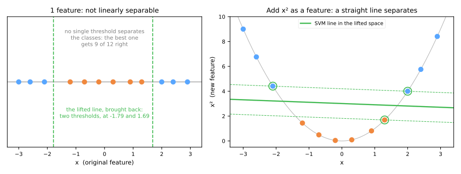
Uma reta no espaço novo \((x, x^2)\) é uma condição de parábola no antigo, \(w_1 x + w_2 x^2 + b > 0\); aqui ela vira dois limiares, em −1,79 e 1,69. É exatamente a ideia dos atributos polinomiais: um modelo linear num espaço de atributos mais rico é um modelo não linear no original.
O problema é o tamanho. Com \(d\) atributos, todos os monômios até o grau \(p\) somam \(\binom{d+p}{p}\):
from math import comb

for d, p in [(2, 2), (34, 3), (784, 3)]:
    print(f"d = {d:3d}, degree {p}: {comb(d + p, p):>11,} monomials")
d =   2, degree 2:           6 monomials
d =  34, degree 3:       7,770 monomials
d = 784, degree 3:  80,931,145 monomials
Com 784 pixels (uma imagem 28 × 28) e grau 3, o mapa explícito tem mais de 80 milhões de colunas.
O kernel: um produto interno sem o mapa
O problema dual e a previsão tocam os dados apenas por meio de produtos internos \(x_i^\top x_j\):
Então, se mapeamos \(x \to \phi(x)\), tudo de que precisamos é \(\langle \phi(x_i), \phi(x_j) \rangle\). Um kernel é uma função que devolve esse número diretamente a partir dos vetores originais:
Conferência numérica, kernel polinomial de grau 2. Para dois atributos, \(\phi(v) = (v_1^2,\ \sqrt2\, v_1 v_2,\ v_2^2)\). Tome \(u = (1, 2)\) e \(v = (3, 1)\):
- pelo mapa: \(\phi(u) = (1,\ 2\sqrt2,\ 4)\), \(\phi(v) = (9,\ 3\sqrt2,\ 1)\), então \(\phi(u) \cdot \phi(v) = 9 + 12 + 4 = 25\);
- pelo kernel: \(u \cdot v = 3 + 2 = 5\), então \(K(u, v) = (u \cdot v)^2 = 25\).
from sklearn.metrics.pairwise import polynomial_kernel

u, v = np.array([1.0, 2.0]), np.array([3.0, 1.0])
phi = lambda z: np.array([z[0] ** 2, np.sqrt(2) * z[0] * z[1], z[1] ** 2])
print("phi(u)·phi(v) =", round(phi(u) @ phi(v), 6))
print("(u·v)^2       =", (u @ v) ** 2)
print("scikit-learn  =", polynomial_kernel([u], [v], degree=2, gamma=1, coef0=0)[0, 0])
O kernel custa um produto escalar de 2 termos e um quadrado, por maior que seja o número de monômios do mapa. Esse é o truque do kernel: a maquinaria linear (margem, hinge, vetores de suporte) num espaço de atributos enorme, ao custo de calcular \(K\) entre pares de pontos no espaço original.
| Kernel | \(K(u, v)\) | Notas |
|---|---|---|
| linear | \(u^\top v\) | a SVM da parte fundamental; o melhor para dados esparsos de alta dimensão (texto) |
| polinomial | \((\gamma\, u^\top v + r)^p\) | todas as interações de atributos até o grau \(p\); coef0 \(= r\) |
| RBF (gaussiano) | \(\exp(-\gamma \lVert u - v \rVert^2)\) | o padrão; seu espaço de atributos tem dimensão infinita |
Um detalhe do kernel polinomial: o padrão do scikit-learn, coef0=0, mantém só os termos de grau exatamente \(p\) (como na conferência acima). Com coef0=1, todos os graus menores também entram, que é o que você normalmente quer.
O kernel RBF é uma semelhança
O kernel RBF vale 1 quando \(u = v\) e decai para 0 com a distância; o \(\gamma\) define a velocidade. Três pontos numa reta, em 0, 1 e 3:
from sklearn.metrics.pairwise import rbf_kernel

P = np.array([[0.0, 0.0], [1.0, 0.0], [3.0, 0.0]])
for gamma in [0.1, 0.5, 2]:
    K = rbf_kernel(P, gamma=gamma)
    print(f"gamma = {gamma:<3}: K(0, 1) = {K[0, 1]:.3f} · K(0, 3) = {K[0, 2]:.5f}")
gamma = 0.1: K(0, 1) = 0.905 · K(0, 3) = 0.40657
gamma = 0.5: K(0, 1) = 0.607 · K(0, 3) = 0.01111
gamma = 2  : K(0, 1) = 0.135 · K(0, 3) = 0.00000
À mão para \(\gamma = 0{,}5\): \(e^{-0{,}5 \cdot 1} = 0{,}607\) e \(e^{-0{,}5 \cdot 9} = 0{,}011\). Com \(\gamma = 0{,}1\), um ponto a 3 unidades ainda conta como bem parecido (0,407); com \(\gamma = 2\), até um ponto a 1 unidade mal conta (0,135) e um a 3 unidades não conta nada.
Agora releia a previsão com esse kernel:
É uma votação ponderada dos vetores de suporte perto de \(x\): cada um vota na sua classe \(y_i\), com um peso que some com a distância. É o k-NN com duas mudanças: o voto é suave (em vez de "os k mais próximos, por igual") e só os vetores de suporte votam, com pesos \(\alpha_i\) aprendidos pela otimização da margem. O \(\gamma\) tem um papel parecido com o de \(1/k\): \(\gamma\) grande significa que só pontos muito próximos importam.
Kernels comparados, medido
Dois conjuntos que nenhuma reta separa, três kernels, CV 5-fold:
from sklearn.datasets import make_circles, make_moons
from sklearn.pipeline import make_pipeline
from sklearn.preprocessing import StandardScaler

datasets = {'circles': make_circles(n_samples=200, factor=0.4, noise=0.12, random_state=0),
            'moons': make_moons(n_samples=200, noise=0.25, random_state=0)}
kernels = {'linear': SVC(kernel='linear'),
           'poly, degree 3': SVC(kernel='poly', degree=3, coef0=1),
           'RBF': SVC(kernel='rbf')}
table = {dname: {kname: cross_val_score(make_pipeline(StandardScaler(), k), Xd, yd, cv=cv).mean()
                 for kname, k in kernels.items()}
         for dname, (Xd, yd) in datasets.items()}
print(pd.DataFrame(table).round(3))
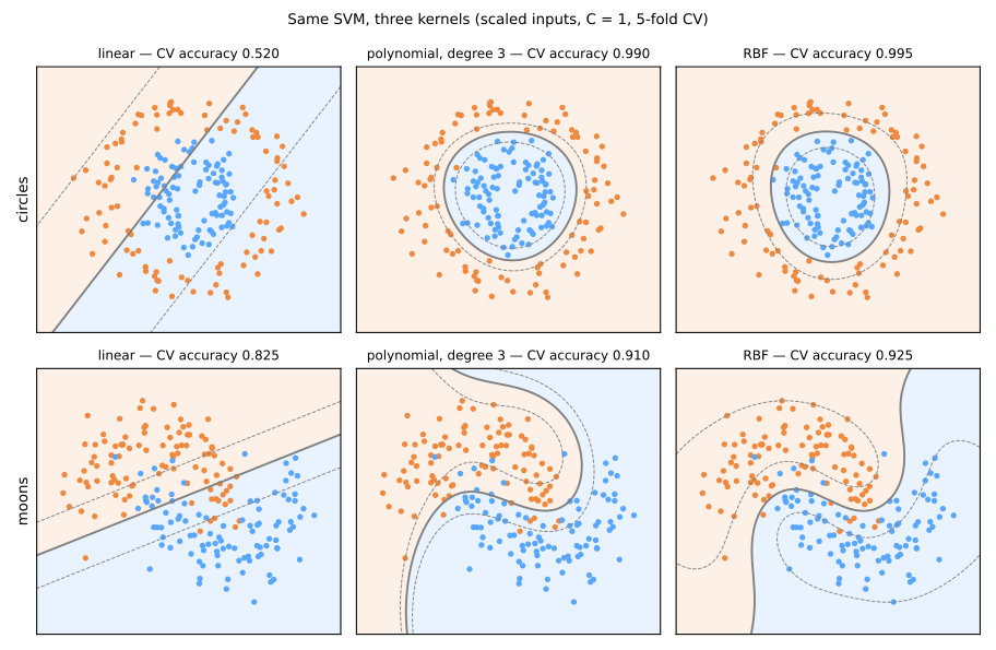
Nos círculos, a SVM linear está no acaso (0,520): nenhuma reta ajuda. Os dois kernels não lineares desenham o anel. Nas luas, o kernel linear ainda chega a 0,825 (uma reta capta a tendência geral); o kernel RBF alcança 0,925 seguindo o vão curvo. O kernel RBF é o padrão do scikit-learn porque raramente vai mal; o kernel linear continua sendo a primeira tentativa certa quando há muitos atributos, como em texto.
6. C e γ juntos
Etapa 2. Com o kernel RBF há dois hiperparâmetros, que interagem:
- \(\gamma\) é o alcance de cada vetor de suporte. \(\gamma\) pequeno: cada vetor de suporte influencia uma região larga e a fronteira é quase linear. \(\gamma\) grande: cada vetor de suporte influencia só a vizinhança imediata e a fronteira pode contornar pontos individuais;
- \(C\) é, como antes, o preço de uma violação da margem.
Eles são ajustados juntos numa grade logarítmica, com um scaler dentro de um pipeline e validação cruzada, exatamente o procedimento da aula de validação:
from sklearn.model_selection import GridSearchCV

X, y = make_moons(n_samples=300, noise=0.3, random_state=1)
grid = GridSearchCV(make_pipeline(StandardScaler(), SVC()),
                    {'svc__C': [0.01, 0.1, 1, 10, 100, 1000],
                     'svc__gamma': [0.01, 0.1, 1, 10, 100, 1000]}, cv=cv)
grid.fit(X, y)
res = pd.DataFrame(grid.cv_results_)
print(res.pivot(index='param_svc__C', columns='param_svc__gamma', values='mean_test_score').round(3))
print(grid.best_params_, f"CV accuracy {grid.best_score_:.3f} ± {res.loc[grid.best_index_, 'std_test_score']:.3f}")
param_svc__gamma  0.01     0.10     1.00     10.00    100.00   1000.00
param_svc__C
0.01                0.830    0.837    0.863    0.897    0.723    0.550
0.10                0.830    0.837    0.870    0.897    0.723    0.550
1.00                0.843    0.837    0.920    0.897    0.840    0.570
10.00               0.830    0.857    0.917    0.877    0.823    0.583
100.00              0.833    0.890    0.903    0.860    0.823    0.583
1000.00             0.837    0.913    0.903    0.860    0.823    0.583
{'svc__C': 1, 'svc__gamma': 1} CV accuracy 0.920 ± 0.022
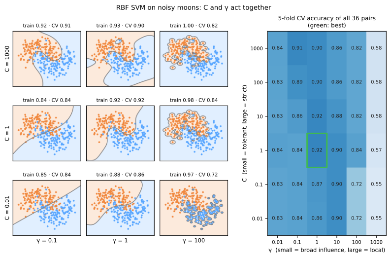
Três regiões para reconhecer, na tabela e na figura:
- Subajuste (colunas da esquerda, \(\gamma = 0{,}01\)): cada vetor de suporte alcança o plano inteiro, então a fronteira é quase uma reta e a acurácia fica presa em 0,83–0,84 para todo \(C\). O painel de baixo à esquerda (\(C = 0{,}01\), \(\gamma = 0{,}1\)) é praticamente a SVM linear.
- Sobreajuste (coluna da direita da tabela, \(\gamma = 1000\); nos painéis, a coluna \(\gamma = 100\)): cada vetor de suporte é uma ilha. A acurácia de treino já é 0,97–1,00 com \(\gamma = 100\) (coluna direita de painéis), mas um ponto novo fica longe de todas as ilhas, recebe \(f(x) \approx b\) e cai numa classe só; a acurácia em CV desaba para 0,55–0,58, pouco acima do baseline de 50%. Com \(\gamma = 100\) e \(C\) pequeno, o painel mostra as ilhas em torno de uma das classes.
- A boa diagonal: as melhores células formam uma crista que vai de \(C\) grande com \(\gamma\) pequeno (0,913 em \(C = 1000\), \(\gamma = 0{,}1\)), passa pelo vencedor (0,920 em \(C = 1\), \(\gamma = 1\)) e chega a \(C\) pequeno com \(\gamma\) maior (0,897 em \(C \leq 1\), \(\gamma = 10\)). Os dois botões trocam flexibilidade por suavidade, então um pouco menos de um pode ser compensado por um pouco mais do outro. É por isso que precisam ser buscados juntos: ajustar o \(C\) com um \(\gamma\) fixo e mal escolhido só encontra a melhor célula de uma coluna ruim.
Como na aula de validação, leia o vencedor com o seu ruído: o desvio-padrão entre folds é 0,022; toda célula a partir de 0,898 (0,917, 0,913, 0,903, …) está a menos de um desvio-padrão dele. "\(C = 1, \gamma = 1\)" é uma boa escolha, não um ótimo comprovado.
7. Escalonar é obrigatório
O kernel RBF mede distância euclidiana ao quadrado, assim como a margem: um atributo medido em milhares domina um medido em frações, exatamente como no k-NN. Medido em dois conjuntos cujos atributos têm dispersões muito diferentes, com e sem um StandardScaler no pipeline:
from sklearn.datasets import load_breast_cancer, load_wine

for name, loader in [('wine', load_wine), ('breast cancer', load_breast_cancer)]:
    Xd, yd = loader(return_X_y=True)
    raw = cross_val_score(SVC(), Xd, yd, cv=cv).mean()
    scaled = cross_val_score(make_pipeline(StandardScaler(), SVC()), Xd, yd, cv=cv).mean()
    print(f"{name:13s} feature std from {Xd.std(0).min():.3f} to {Xd.std(0).max():5.1f} · "
          f"raw {raw:.3f} · scaled {scaled:.3f}")
wine          feature std from 0.124 to 314.0 · raw 0.657 · scaled 0.983
breast cancer feature std from 0.003 to 568.9 · raw 0.921 · scaled 0.977
No wine, um atributo (a prolina, na casa das centenas) tem desvio-padrão mais de 2.500 vezes maior que o do menor. Sem escalonar, o kernel enxerga quase só a prolina e a acurácia é 0,657; escalonado, 0,983. O padrão gamma='scale' não resolve isso: ele divide pela variância de todos os atributos juntos, então adapta o \(\gamma\) à escala geral, mas não às diferenças entre atributos. O scaler vai dentro do pipeline, para que cada fold da CV ajuste o seu próprio scaler nas suas próprias linhas de treino.
8. Escores e probabilidades
decision_function basta para a ROC
Etapa 3. A saída natural de uma SVM é o escore \(f(x)\), disponível como decision_function. O sinal dele é a previsão; o valor é uma distância com sinal até a fronteira, em unidades de meia margem: \(\pm 1\) nas bordas da rua. Não é uma probabilidade, mas ordena os pontos — e ordenar é tudo de que a ROC AUC e a precisão média precisam.
Quando você precisa mesmo de probabilidades (para combinar com custos ou reportar um risco), a solução padrão é o escalonamento de Platt (Platt, 1999): ajustar uma regressão logística de um atributo só, \(P(y = 1 \mid x) = 1 / (1 + e^{A f(x) + B})\), sobre escores obtidos por validação cruzada interna e depois reajustar a SVM em todos os dados. SVC(probability=True) sempre fez isso internamente; desde o scikit-learn 1.9 ele está marcado como obsoleto (deprecated) em favor do equivalente explícito CalibratedClassifierCV(..., method='sigmoid', ensemble=False), que também funciona em versões antigas:
from sklearn.calibration import CalibratedClassifierCV
from sklearn.metrics import roc_auc_score
from sklearn.model_selection import train_test_split

Xd, yd = load_breast_cancer(return_X_y=True)
X_tr, X_te, y_tr, y_te = train_test_split(Xd, yd, test_size=0.25, stratify=yd, random_state=0)

svm = make_pipeline(StandardScaler(), SVC()).fit(X_tr, y_tr)
platt = CalibratedClassifierCV(make_pipeline(StandardScaler(), SVC()), method='sigmoid',
                               ensemble=False, cv=cv).fit(X_tr, y_tr)
f, p = svm.decision_function(X_te), platt.predict_proba(X_te)[:, 1]
print(f"ROC AUC from f(x): {roc_auc_score(y_te, f):.4f} · from Platt probabilities: {roc_auc_score(y_te, p):.4f}")

near = np.argsort(np.abs(f))[:3]                          # os três pontos de teste mais próximos de f = 0
print(pd.DataFrame({'f(x)': f[near].round(3), 'P(y=1)': p[near].round(3),
                    'SVC predicts': svm.predict(X_te[near]), 'Platt predicts': platt.predict(X_te[near])}))
print("disagreements on the test set:", (svm.predict(X_te) != platt.predict(X_te)).sum(), "of", len(y_te))
ROC AUC from f(x): 0.9927 · from Platt probabilities: 0.9927
    f(x)  P(y=1)  SVC predicts  Platt predicts
0 -0.001   0.451             0               0
1  0.043   0.494             1               0
2  0.104   0.554             1               1
disagreements on the test set: 1 of 143
Duas coisas para notar:
- A ROC AUC é idêntica até a quarta casa. A sigmoide de Platt é monótona, então preserva a ordem dos escores; as probabilidades acrescentam calibração, não discriminação. Para ROC, curvas de precisão–recall ou escolha de limiar em escores de validação, a
decision_functionbasta e não exige ajustes extras. - Os dois podem discordar perto da fronteira. O ponto com \(f(x) = 0{,}043\) é classe 1 para a SVM (escore positivo), mas recebe \(P = 0{,}494\), classe 0 para o modelo calibrado, porque a sigmoide ajustada não fica centrada exatamente em \(f = 0\). Um ponto de teste em 143, aqui. E custa ajustes extras: 5 ajustes da CV interna mais o final.
Classes desbalanceadas: class_weight
class_weight='balanced' multiplica a perda hinge de cada ponto pelo inverso da frequência da sua classe, exatamente como na aula de dados desbalanceados; na SVM isso significa um \(C\) separado por classe. Medido num problema sintético com 10% de positivos:
from sklearn.datasets import make_classification
from sklearn.model_selection import cross_validate

Xd, yd = make_classification(n_samples=1000, weights=[0.9], n_features=10, n_informative=4,
                             flip_y=0.03, random_state=0)
for cw in [None, 'balanced']:
    r = cross_validate(make_pipeline(StandardScaler(), SVC(class_weight=cw)), Xd, yd, cv=cv,
                       scoring=['recall', 'precision', 'balanced_accuracy', 'roc_auc'])
    print(f"class_weight={str(cw):9s}", " · ".join(f"{k[5:]} {v.mean():.3f}" for k, v in r.items()
                                                  if k.startswith('test_')))
class_weight=None      recall 0.181 · precision 0.893 · balanced_accuracy 0.589 · roc_auc 0.838
class_weight=balanced  recall 0.578 · precision 0.379 · balanced_accuracy 0.727 · roc_auc 0.809
O recall da classe minoritária sobe de 0,181 para 0,578 e a precisão cai de 0,893 para 0,379: a mesma troca de mover o limiar, paga com um modelo reajustado. A ROC AUC não melhora; chega a cair (de 0,838 para 0,809). Reponderar não é mover o limiar: o modelo é reajustado, o que desloca a fronteira a favor da classe minoritária e pode ordenar os escores um pouco pior no conjunto.
9. Multiclasse: um-contra-um
A SVM é um método de duas classes. A SVC lida com \(k\) classes por um-contra-um (one-vs-one): treina uma SVM binária para cada par de classes (\(k(k-1)/2\) delas) e prevê por votação da maioria. No conjunto de 10 dígitos (imagens 8 × 8, 64 atributos de pixel):
from sklearn.datasets import load_digits
from sklearn.svm import LinearSVC

Xd, yd = load_digits(return_X_y=True)
ovo = SVC(decision_function_shape='ovo').fit(Xd, yd)
print("pairwise classifiers:", ovo.decision_function(Xd[:1]).shape[1], "= 10·9/2")
print("support vectors per digit:", ovo.n_support_, "· total", ovo.n_support_.sum(), "of", len(Xd))
print("LinearSVC (one-vs-rest) coefficients:", LinearSVC().fit(Xd, yd).coef_.shape)
print(f"CV accuracy · raw pixels {cross_val_score(SVC(), Xd, yd, cv=cv).mean():.3f} · "
      f"scaled {cross_val_score(make_pipeline(StandardScaler(), SVC()), Xd, yd, cv=cv).mean():.3f}")
pairwise classifiers: 45 = 10·9/2
support vectors per digit: [ 45  94  66  78  62  77  52  72 106  95] · total 747 of 1797
LinearSVC (one-vs-rest) coefficients: (10, 64)
CV accuracy · raw pixels 0.987 · scaled 0.981
São 45 classificadores de pares, cada um treinado só nas linhas dos seus dois dígitos (cerca de um quinto dos dados), o que sai mais barato do que parece para um método cujo custo cresce mais rápido que \(n\). Por padrão, predict e decision_function apresentam o resultado com uma coluna por classe (decision_function_shape='ovr'), mas por baixo continua sendo um-contra-um. A LinearSVC usa um-contra-o-resto (one-vs-rest): 10 classificadores, uma linha de 64 coeficientes cada.
A última linha refina o "escalonar é obrigatório": os pixels estão todos na mesma unidade (0–16 níveis de cinza), então não há nada a igualar; padronizar chega a custar um pouco (0,987 cru contra 0,981 escalonado), muito provavelmente porque infla pixels quase constantes da borda até o mesmo peso dos informativos. A regra é "pôr todos os atributos numa escala comparável"; o StandardScaler é o jeito usual, não o único.
10. Custo: quando as SVMs deixam de ser práticas
Tempo de treino
Etapa 4. Uma SVM com kernel precisa do kernel entre pares de pontos de treino, cujo número cresce como \(n^2\). Na prática, os solvers levam entre cerca de \(n^2\) e \(n^3\) operações, dependendo de quantos pontos terminam como vetores de suporte (script da figura):
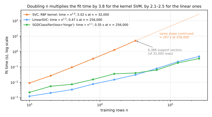
Os tempos absolutos dependem da máquina que rodou o script; as inclinações, não. Cada vez que \(n\) dobra, o tempo de ajuste da SVM com kernel é multiplicado por cerca de 3,8 (inclinação 1,9 no gráfico log-log). Com 32.000 linhas ela leva cerca de 5 segundos e guarda mais de 6.000 vetores de suporte, o que também deixa a previsão lenta: cada ponto novo exige uma avaliação do kernel contra cada um deles. Seguindo a mesma inclinação, 256.000 linhas levariam cerca de 4,5 minutos, para um ajuste de um par \((C, \gamma)\); uma grade de 25 células com CV 5-fold multiplica isso por 125.
Para SVMs lineares existem solvers especializados que nunca montam a matriz de kernel: a LinearSVC (liblinear) e o SGDClassifier(loss='hinge'), que minimiza o mesmo objetivo hinge + L2 por gradiente descendente estocástico. Os dois ajustam 256.000 linhas em menos de meio segundo na figura. Quão perto chegam de SVC(kernel='linear')? Nos dígitos:
from sklearn.linear_model import SGDClassifier
from sklearn.multiclass import OneVsOneClassifier, OneVsRestClassifier

linear_models = {'SVC(kernel="linear")': SVC(kernel='linear'),
                 'LinearSVC()': LinearSVC(),
                 'SGDClassifier(hinge)': SGDClassifier(loss='hinge', random_state=0),
                 'SVC, one-vs-rest': OneVsRestClassifier(SVC(kernel='linear')),
                 'LinearSVC, one-vs-one': OneVsOneClassifier(LinearSVC())}
for name, model in linear_models.items():
    acc = cross_val_score(make_pipeline(StandardScaler(), model), Xd, yd, cv=cv).mean()
    print(f"{name:22s} CV accuracy on digits {acc:.3f}")
SVC(kernel="linear")   CV accuracy on digits 0.979
LinearSVC()            CV accuracy on digits 0.955
SGDClassifier(hinge)   CV accuracy on digits 0.949
SVC, one-vs-rest       CV accuracy on digits 0.952
LinearSVC, one-vs-one  CV accuracy on digits 0.979
Os solvers especializados ficam 2–3 pontos atrás (0,955 e 0,949 contra 0,979), e as duas últimas linhas mostram que o motivo não é o solver. Com dez classes, a SVC treina um-contra-um (45 classificadores por par, seção 9), enquanto a LinearSVC e o SGDClassifier treinam um-contra-o-resto: 10 classificadores, cada um separando um dígito dos outros nove. Forçada a um-contra-o-resto, a SVC cai para 0,952; embrulhada em um-contra-um, a LinearSVC sobe para 0,979. Uma reta separa dois dígitos com mais facilidade do que um dígito de todos os outros. As demais diferenças pesam menos aqui: por padrão, a LinearSVC usa a hinge ao quadrado e também penaliza o intercepto; o SGDClassifier faz passadas estocásticas (ruidosas) pelos dados, com o seu próprio parâmetro de regularização alpha no lugar do C, então cada um precisa do seu próprio ajuste. O que os solvers especializados ganham é escala. Uma regra prática a partir dessas medições: uma SVM com kernel vai bem até algumas dezenas de milhares de linhas; além disso, use uma SVM linear sobre atributos bem escolhidos ou modelos que escalam melhor, como o gradient boosting.
Como ela é treinada, em essência
Os solvers otimizam o dual (ex.: SMO — Sequential Minimal Optimization, Platt 1998 — que otimiza pares de \(\alpha_i\) até valerem as condições de otimalidade, chamadas KKT (Karush–Kuhn–Tucker); a libsvm, por trás da SVC, usa uma versão refinada). Um esboço em pseudocódigo da ideia:
inicialize todos os α_i = 0
repita até as condições KKT valerem (dentro da tolerância):
    escolha um par (α_i, α_j) que viole as condições      # escolha heurística
    otimize o objetivo sobre esse par analiticamente       # forma fechada para 2 variáveis
    limite a 0 ≤ α ≤ C, atualize b
os pontos que terminam com α_i > 0 são os vetores de suporte
Regressão: SVR
As mesmas ideias dão um regressor, a SVR: ela ajusta uma função com um tubo de meia largura \(\varepsilon\) em volta, ignora resíduos menores que \(\varepsilon\) (o análogo, na regressão, de "além da margem") e paga linearmente pelo resto. Kernels, \(C\), \(\gamma\), escalonamento e custo se comportam exatamente como na classificação.
11. Perfil prático
| SVM (kernel RBF) | Regressão logística | k-NN | |
|---|---|---|---|
| Fronteira | qualquer forma suave (kernel) | linear nos atributos | qualquer forma, local |
| Perda | hinge: ignora pontos além da margem | log loss: todo ponto conta | nenhuma (não há treino) |
| O que guarda | os vetores de suporte e seus \(\alpha_i\) | \(w, b\) | o conjunto de treino inteiro |
| Hiperparâmetros | \(C\) e \(\gamma\), acoplados | \(C\) | \(k\), distância |
| Precisa escalonar | sim | sim (pela penalidade e pelo solver) | sim |
| Probabilidades | não; escalonamento de Platt depois | sim, nativas | frações de voto (grosseiras) |
| Custo de treino | \(\sim n^2\) a \(n^3\) | \(\sim n\) | nenhum |
| Custo de previsão | um kernel por vetor de suporte | um produto escalar | distâncias às \(n\) linhas |
| Interpretabilidade | baixa (exceto kernel linear) | alta: coeficientes, chances | média: "estes vizinhos" |
| Recorra a ela quando | \(n\) pequeno/médio, fronteira não linear, muitos atributos | precisa de probabilidades ou explicações ou tem \(n\) grande | problemas minúsculos e de baixa dimensão, baselines rápidos |
Lab avançado — o kernel e o ajuste
Os passos 5 a 9 ligam o kernel RBF no mesmo problema de radar, ajustam \(C\) e \(\gamma\) juntos, abrem o vencedor e o medem uma única vez no conjunto de teste trancado no passo 2.
Como fazer este lab em aula (cerca de 35 min, em duplas)
- Use o mesmo notebook do Colab do lab fundamental e vá até o passo 5. Nada para baixar.
- Os passos 5 a 9 usam os objetos dos passos 2 a 4 (
X_train,cv,cv_summary,models). Se a sessão do Colab for nova (ou tiver expirado), clique na célula do passo 5 e use Ambiente de execução → Executar anteriores (Ctrl+F8) antes de continuar. - A dinâmica é a mesma: Preveja antes de rodar, compare com a página e tente as Simulações antes de abrir a solução.
- Ritmo sugerido: passos 5 e 6 com a simulação em 15 min; passo 7 e a simulação em 10 min; passos 8 e 9 em 10 min.
Passo 5 — ligar o kernel RBF
Preveja. A única mudança é kernel='rbf', sem ajuste nenhum. O ganho sobre a SVM linear vai ser maior ou menor que o desvio entre folds do passo 4 (cerca de 0,02)?
rbf = make_pipeline(StandardScaler(), SVC(kernel='rbf'))       # padrões: C = 1, gamma = 'scale'
print(cv_summary(rbf))

Z = StandardScaler().fit_transform(X_train)
print(f"gamma='scale' means gamma = 1 / (n_features · variance) = {1 / (Z.shape[1] * Z.var()):.4f}")
{'accuracy': '0.939 ± 0.022', 'roc_auc': '0.988 ± 0.007'}
gamma='scale' means gamma = 1 / (n_features · variance) = 0.0303
Trocar o kernel de linear para RBF, sem ajuste nenhum, leva a acurácia de 0,886 para 0,939 e a ROC AUC de 0,850 para 0,988. O ganho de acurácia, 5,3 pontos, é mais que o dobro do desvio-padrão entre folds. Esse é o efeito do kernel, muito maior que as diferenças entre os três modelos do passo 4.
A segunda linha decifra o gamma='scale'. Depois de padronizar, 33 colunas têm variância 1 e a constante tem 0, então a variância conjunta é \(33/34\) e \(\gamma = 1 / (34 \cdot 33/34) = 1/33 = 0{,}0303\). Um padrão razoável, mas só um padrão: o passo 6 busca em volta dele.
Passo 6 — ajustar C e γ juntos
Preveja. Numa grade de 25 pares \((C, \gamma)\), você espera que o melhor valor de \(C\) dependa do \(\gamma\) escolhido? E qual canto da tabela deve ser o pior: \(\gamma\) muito pequeno ou muito grande?
import matplotlib.pyplot as plt
from sklearn.model_selection import GridSearchCV

param_grid = {'svc__C': [0.1, 1, 10, 100, 1000],
              'svc__gamma': [0.0001, 0.001, 0.01, 0.1, 1]}
grid = GridSearchCV(rbf, param_grid, cv=cv, scoring='accuracy', return_train_score=True)
grid.fit(X_train, y_train)

res = pd.DataFrame(grid.cv_results_)
table = res.pivot(index='param_svc__C', columns='param_svc__gamma', values='mean_test_score')
print(table.round(3))
best_std = res.loc[grid.best_index_, 'std_test_score']
print(f"best: {grid.best_params_} · accuracy {grid.best_score_:.3f} ± {best_std:.3f}")
ties = res[res['mean_test_score'] >= grid.best_score_ - best_std]
print(f"{len(ties)} of {len(res)} pairs are within one std of the best")
corner = (res['param_svc__C'] == 1) & (res['param_svc__gamma'] == 1)
print(f"training-fold accuracy · best pair {res.loc[grid.best_index_, 'mean_train_score']:.3f} · "
      f"C = 1, gamma = 1: {res.loc[corner, 'mean_train_score'].item():.3f}")

plt.imshow(table, cmap='Blues', origin='lower')
plt.xticks(range(5), table.columns); plt.yticks(range(5), table.index)
plt.xlabel('gamma'); plt.ylabel('C'); plt.colorbar(label='CV accuracy')
plt.show()
param_svc__gamma  0.0001  0.0010  0.0100  0.1000  1.0000
param_svc__C
0.1                0.643   0.643   0.719   0.643   0.643
1.0                0.643   0.757   0.916   0.954   0.665
10.0               0.753   0.894   0.932   0.951   0.669
100.0              0.878   0.920   0.939   0.954   0.669
1000.0             0.882   0.920   0.932   0.954   0.669
best: {'svc__C': 1, 'svc__gamma': 0.1} · accuracy 0.954 ± 0.019
5 of 25 pairs are within one std of the best
training-fold accuracy · best pair 0.991 · C = 1, gamma = 1: 1.000
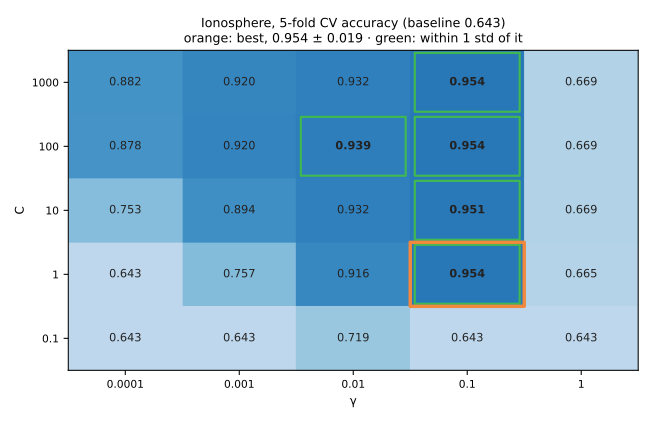
Leia a tabela como um mapa de três regiões:
- Regularizado demais (primeira linha da tabela, \(C = 0{,}1\); coluna \(\gamma = 0{,}0001\) com \(C\) pequeno): acurácia 0,643, exatamente o baseline, em cinco dessas células; na primeira linha só \(\gamma = 0{,}01\) escapa, e por pouco (0,719). A margem é tão barata de violar que a SVM desiste e prevê a classe majoritária.
- Local demais (coluna da direita, \(\gamma = 1\)): 0,665–0,669, pouco acima do baseline, para todo \(C \geq 1\). Cada vetor de suporte só influencia uma bolinha em volta de si, um retorno novo fica longe de todos eles, recebe \(f(x) \approx b\) e é chamado de "bom". Enquanto isso, os folds de treino são ajustados perfeitamente (1,000 com \(C = 1\), última linha da saída, contra 0,991 do vencedor): o canto clássico do sobreajuste.
- A crista: as melhores células ficam em \(\gamma = 0{,}1\) (e em \(\gamma = 0{,}01\) com \(C\) grande).
O vencedor é \(C = 1\), \(\gamma = 0{,}1\), com 0,954 ± 0,019. Três células imprimem 0,954 (\(C\) = 1, 100 e 1000 com \(\gamma = 0{,}1\)); o GridSearchCV fica com a primeira que encontrou, que é também a mais regularizada, um desempate sensato. Cinco dos 25 pares estão a menos de um desvio-padrão do melhor (verdes na figura): quatro com \(\gamma = 0{,}1\), com \(C\) em qualquer valor de 1 a 1000, e um com \(\gamma = 0{,}01\) e \(C = 100\) (0,939). Neste conjunto, o \(\gamma\) é o botão que importa. Note também o tamanho do ganho: o ajuste levou a acurácia de 0,939 (padrões) para 0,954, menos de um desvio-padrão, enquanto ligar o kernel a tinha movido 5,3 pontos.
Simulação: o que o γ faz, visto de dentro. Fixe C = 1 e varra o \(\gamma\) de 0,001 a 1. Para cada valor, conte os vetores de suporte e compare a acurácia de treino com a de validação cruzada. O vão entre as duas conta a história do sobreajuste melhor que qualquer um dos números sozinho.
Solução
from sklearn.model_selection import cross_val_score

print("gamma   vetores de suporte   com α = C   treino      CV   vão")
for gamma in [0.001, 0.01, 0.1, 1]:
    m = make_pipeline(StandardScaler(), SVC(gamma=gamma, C=1)).fit(X_train, y_train)
    at_C = (np.abs(m[-1].dual_coef_) >= 1 - 1e-6).sum()       # alpha = C: dentro da rua ou do lado errado
    tr = m.score(X_train, y_train)
    acc = cross_val_score(make_pipeline(StandardScaler(), SVC(gamma=gamma, C=1)),
                          X_train, y_train, cv=cv).mean()
    print(f"{gamma:<8g}{m[-1].n_support_.sum():18d}{at_C:12d}{tr:9.3f}{acc:8.3f}{tr - acc:6.3f}")
gamma   vetores de suporte   com α = C   treino      CV   vão
0.001                  184         178    0.802   0.757 0.046
0.01                   109          83    0.943   0.916 0.027
0.1                    148          29    0.989   0.954 0.034
1                      231          87    1.000   0.665 0.335
O número de vetores de suporte faz um U, e a coluna \(\alpha = C\) mostra que os dois braços têm causas diferentes. À esquerda, com \(\gamma = 0{,}001\), cada vetor de suporte alcança o conjunto inteiro, a fronteira é quase linear e o modelo subajusta (acurácia de treino de só 0,802): 178 dos seus 184 vetores de suporte têm \(\alpha = C\), ou seja, não são pontos de que a fronteira precisa, são violações da margem, linhas dentro da rua ou do lado errado. No meio, o kernel descreve a fronteira com menos pontos (109 e 148), e em \(\gamma = 0{,}1\) a maioria deles (119 de 148) fica exatamente sobre a margem. À direita, com \(\gamma\) grande demais, cada ponto vira uma ilha e quase toda linha de treino precisa ser guardada (231 de 263). O vão treino − CV é o detector de sobreajuste: 0,027 e 0,034 na faixa boa e 0,335 em \(\gamma = 1\), em que o treino é perfeito e a CV desaba para 0,665, logo acima do baseline de 0,643. Em \(\gamma = 0{,}001\) o vão é pequeno (0,046), mas os dois números são baixos: o subajuste não aparece no vão, só no nível. Decorar os dados de treino e não generalizar nada é exatamente o que "cada vetor de suporte é uma ilha" significa.
Passo 7 — por dentro do vencedor: os vetores de suporte
Preveja. O vencedor tem \(\gamma = 0{,}1\), razoavelmente local, em 34 dimensões. Você espera que ele guarde uns 10% das linhas de treino como vetores de suporte ou bem mais?
best = grid.best_estimator_                     # reajustado em todo o X_train
svc = best[-1]
print(f"support vectors (bad, good): {svc.n_support_} · {svc.n_support_.sum()} of {len(X_train)} rows")

alpha = np.abs(svc.dual_coef_[0])
print(f"on the margin (0 < alpha < C): {(alpha < svc.C - 1e-6).sum()} · "
      f"inside it or misclassified (alpha = C): {(alpha >= svc.C - 1e-6).sum()}")

m = np.where(y_train == 1, 1, -1) * best.decision_function(X_train)   # m = y · f(x)
print(f"training rows with m < 0 (misclassified): {(m < 0).sum()} · "
      f"training accuracy {best.score(X_train, y_train):.3f}")
support vectors (bad, good): [91 57] · 148 of 263 rows
on the margin (0 < alpha < C): 119 · inside it or misclassified (alpha = C): 29
training rows with m < 0 (misclassified): 3 · training accuracy 0.989
148 das 263 linhas de treino (56%) são vetores de suporte, muito mais que nos exemplos de brinquedo. Isso é típico de um kernel RBF bastante local em 34 dimensões e define o custo de previsão do modelo: cada retorno novo é comparado com 148 guardados. A divisão por classe chama a atenção: 91 dos 94 retornos ruins são vetores de suporte, contra 57 dos 169 bons. Os retornos bons ocupam uma região que o kernel consegue descrever com um terço dos seus pontos; quase todo retorno ruim é necessário, o que é coerente com os retornos ruins serem mais variados.
Os coeficientes duais separam os vetores de suporte como na seção de margem suave: 119 ficam exatamente sobre a margem (\(0 < \alpha_i < C\)) e 29 estão dentro da rua ou do lado errado (\(\alpha_i = C\), o máximo que um ponto pode pesar). Só 3 linhas de treino são classificadas errado, então a acurácia de treino é 0,989 contra 0,954 na CV: uma diferença de 3,5 pontos, algum sobreajuste, mas não o colapso da coluna \(\gamma = 1\).
Simulação: escalonar num conjunto que já está normalizado. O passo 1 notou que todos os atributos já estão entre −1 e 1. Então o StandardScaler ainda faz diferença aqui? Meça a acurácia de CV do vencedor com e sem ele e olhe antes a faixa de desvios-padrão das colunas.
Solução
from sklearn.model_selection import cross_val_score

print(f"atributos já vão de {X_train.min().min():.0f} a {X_train.max().max():.0f}; "
      f"desvios de {X_train.std().min():.3f} a {X_train.std().max():.3f}")
for name, model in [('sem scaler', SVC(C=1, gamma=0.1)),
                    ('com StandardScaler', make_pipeline(StandardScaler(), SVC(C=1, gamma=0.1)))]:
    acc = cross_val_score(model, X_train, y_train, cv=cv).mean()
    print(f"{name:20s} CV {acc:.3f}")
atributos já vão de -1 a 1; desvios de 0.000 a 0.655
sem scaler           CV 0.943
com StandardScaler   CV 0.954
Mesmo com tudo já dentro de [−1, 1], padronizar ainda vale 1,1 ponto (0,954 contra 0,943). A faixa de valores comum esconde uma diferença real de dispersão: os desvios-padrão vão de 0,000 (a coluna constante a02) a 0,655, uma razão que o kernel RBF enxerga, porque ele soma diferenças ao quadrado coluna a coluna. Parte do estrago é indireta: com dispersões abaixo de 1, as distâncias encolhem e o \(\gamma = 0{,}1\) — escolhido junto com o scaler — fica efetivamente pequeno demais. Compare com o wine da seção 7, em que a mesma omissão custava 32,6 pontos (0,657 contra 0,983): o tamanho do estrago depende de quão desiguais são as escalas. A conclusão prática é a mesma nos dois casos — o scaler vai dentro do pipeline, porque não custa nada e você não sabe de antemão em qual dos dois mundos está.
Passo 8 — a SVM é mesmo melhor? Rivais ajustados, mesmos folds
Preveja. Agora os rivais também são ajustados. A vantagem da SVM RBF vai sobreviver a isso? E por que o desvio das diferenças por fold deve ser menor que o desvio de cada modelo?
rivals = {
    'logistic regression': GridSearchCV(models['logistic regression'],
                                        {'logisticregression__C': [0.001, 0.01, 0.1, 1, 10, 100, 1000]},
                                        cv=cv),
    'k-NN': GridSearchCV(models['k-NN (k = 5)'],
                         {'kneighborsclassifier__n_neighbors': [1, 3, 5, 7, 9, 15, 25]}, cv=cv),
}


def fold_scores(g):                              # os 5 escores por fold do vencedor de uma grade
    return [g.cv_results_[f'split{k}_test_score'][g.best_index_] for k in range(5)]


folds = pd.DataFrame({'RBF SVM': fold_scores(grid)})
for name, g in rivals.items():
    g.fit(X_train, y_train)
    print(f"{name}: {g.best_params_}")
    folds[name] = fold_scores(g)
folds['SVM - LR'] = folds['RBF SVM'] - folds['logistic regression']
folds['SVM - k-NN'] = folds['RBF SVM'] - folds['k-NN']
print(folds.round(3))
print(pd.DataFrame({'mean': folds.mean(), 'std': folds.std(ddof=0)}).T.round(3))
logistic regression: {'logisticregression__C': 10}
k-NN: {'kneighborsclassifier__n_neighbors': 1}
   RBF SVM  logistic regression   k-NN  SVM - LR  SVM - k-NN
0    0.925                0.868  0.830     0.057       0.094
1    0.962                0.887  0.849     0.075       0.113
2    0.962                0.887  0.887     0.075       0.075
3    0.942                0.904  0.846     0.038       0.096
4    0.981                0.923  0.885     0.058       0.096
      RBF SVM  logistic regression   k-NN  SVM - LR  SVM - k-NN
mean    0.954                0.894  0.859     0.061       0.095
std     0.019                0.019  0.022     0.014       0.012
Cada rival é ajustado do mesmo jeito, nos mesmos folds: a regressão logística fica em \(C = 10\), o k-NN em \(k = 1\) (o ajuste mais local, assim como a SVM também preferiu um \(\gamma\) bastante local). Aí a comparação é feita fold a fold:
- a SVM RBF vence a regressão logística ajustada em todos os cinco folds, por 0,038 a 0,075, média 0,061 ± 0,014;
- vence também o k-NN ajustado nos cinco folds, por 0,075 a 0,113, média 0,095 ± 0,012.
Repare que o desvio-padrão das diferenças (0,012–0,014) é menor que o de cada modelo (0,019–0,022). Um fold difícil para um modelo é difícil para todos; parear nos mesmos folds cancela essa dificuldade compartilhada. É por isso que todos os modelos deste lab usaram o mesmo objeto cv. Uma ressalva: cada coluna é a melhor da sua própria grade, então as três são um pouco otimistas, a SVM (melhor de 25) um pouco mais que as outras (melhor de 7). A CV aninhada, em Sua vez, remove esse viés.
Passo 9 — o único teste
Preveja. A CV disse 0,954 ± 0,019. Com 88 linhas de teste, quanto um único erro vale? Um resultado alguns pontos abaixo da CV seria motivo para voltar e reajustar?
from sklearn.metrics import classification_report, confusion_matrix, roc_auc_score

pred = best.predict(X_test)
print(confusion_matrix(y_test, pred, labels=[1, 0]))
print(classification_report(y_test, pred, target_names=['bad', 'good'], digits=3))
print(f"test ROC AUC (from decision_function): {roc_auc_score(y_test, best.decision_function(X_test)):.3f}")
[[52  4]
 [ 4 28]]
              precision    recall  f1-score   support

         bad      0.875     0.875     0.875        32
        good      0.929     0.929     0.929        56

    accuracy                          0.909        88
   macro avg      0.902     0.902     0.902        88
weighted avg      0.909     0.909     0.909        88

test ROC AUC (from decision_function): 0.956
Uma vez, no fim, a SVM ajustada encontra as 88 linhas de teste: acurácia 0,909 (80 acertos: 4 retornos ruins chamados de bons, 4 bons chamados de ruins) e ROC AUC 0,956. Precisão e recall são 0,875 para a classe ruim e 0,929 para a boa.
Isso fica 4,5 pontos abaixo da estimativa da CV, 0,954 ± 0,019. Tem algo errado? Se a acurácia verdadeira fosse 0,954, 88 linhas de teste teriam um erro-padrão de cerca de \(\sqrt{0{,}954 \times 0{,}046 / 88} \approx 0{,}022\), então 0,909 fica dois erros-padrão abaixo: um sorteio azarado, mas não implausível, ainda mais porque 0,954 já era o melhor de 25 candidatos. A conclusão do passo 8 (a SVM com kernel vence os modelos lineares por cerca de 6 pontos) se apoia em folds pareados e não é derrubada por um conjunto de teste pequeno. O que você não pode fazer agora é voltar ao passo 6 e reajustar até o teste parecer melhor: o conjunto de teste viraria um conjunto de validação e 0,909 deixaria de significar alguma coisa.
Para fechar a aula. Em uma frase cada: (1) o que o truque do kernel evita calcular? (2) Por que \(C\) e \(\gamma\) precisam ser buscados juntos? (3) Quando uma SVM com kernel deixa de ser prática e o que usar no lugar?
Sua vez (avançado)
Para casa, com mais tempo:
- Kernel polinomial. Troque o RBF por
SVC(kernel='poly', coef0=1)e ajustedegree(2, 3, 4) eCcom o mesmocv. Ele chega a menos de um desvio-padrão do vencedor RBF? Quantos vetores de suporte ele guarda? - CV aninhada. Rode
cross_val_score(grid, X_train, y_train, cv=StratifiedKFold(5, shuffle=True, random_state=7)). Esse escore avalia o procedimento de ajuste inteiro em folds que o ajuste nunca viu. Compare comgrid.best_score_e com a acurácia de teste do passo 9: de qual dos dois ele fica mais perto? - Probabilidades. Monte
CalibratedClassifierCV(grid.best_estimator_, method='sigmoid', ensemble=False, cv=cv)e compare a ROC AUC dele em validação cruzada (acv_summaryfunciona com ele) com a do próprio vencedor (cv_summary(grid.best_estimator_)). Por que as duas ficam tão próximas? Depois usecross_val_predictnos dois para contar as linhas de treino cuja classe prevista muda. - Multiclasse. No
load_digits, ajusteCegammadaSVCcom umGridSearchCVe umcvestratificado de 5 folds. Quantos classificadores de pares o vencedor treina e quantos vetores de suporte ele guarda para o dígito 8 comparado ao dígito 0? Quais dígitos são os mais difíceis, segundo a matriz de confusão das previsões fora do fold?
Vídeos
- SVM — Support Vector Machines: Fundamentos e prática — em português
- 16. Learning: Support Vector Machines — MIT OpenCourseWare, Patrick Winston
Leitura complementar
- Wikipedia — Quadratic programming
- Wikipedia — Sequential minimal optimization (SMO)
- Guia do usuário do scikit-learn — Support Vector Machines
Referências
- Boser, B.; Guyon, I.; Vapnik, V. "A Training Algorithm for Optimal Margin Classifiers." COLT (1992). DOI
- Cortes, C.; Vapnik, V. "Support-Vector Networks." Machine Learning 20 (1995). DOI
- Platt, J. "Sequential Minimal Optimization: A Fast Algorithm for Training Support Vector Machines." Microsoft Research Technical Report MSR-TR-98-14 (1998). Link
- Platt, J. "Probabilistic Outputs for Support Vector Machines and Comparisons to Regularized Likelihood Methods." Em Advances in Large Margin Classifiers, MIT Press (1999), 61–74 — o escalonamento de Platt.
- Hsu, C.-W.; Chang, C.-C.; Lin, C.-J. "A Practical Guide to Support Vector Classification." Relatório técnico, National Taiwan University (2003) — escalonar os atributos e depois fazer busca em grade de C e γ em escala logarítmica. PDF
- Sigillito, V. G.; Wing, S. P.; Hutton, L. V.; Baker, K. B. "Classification of Radar Returns from the Ionosphere Using Neural Networks." Johns Hopkins APL Technical Digest 10 (1989), 262–266 — o conjunto de dados do lab.
Quiz
O quiz cobre a abordagem fundamental.