Representação de Texto
Toda técnica vista até aqui no curso parte de uma tabela de números: a PCA gira suas colunas, o k-means mede distâncias entre suas linhas. Texto não chega como tabela. Uma avaliação de cliente, um chamado de suporte, um post de fórum é uma sequência de caracteres de qualquer tamanho. Esta aula constrói a ponte de strings a vetores, para que as ferramentas geométricas que você já conhece (distâncias, projeções, agrupamentos) se apliquem a texto. Ela é também a base da próxima aula, Modelagem de Tópicos & BERTopic, que junta tudo o que está aqui.
Há duas famílias de respostas:
- representações esparsas (bag-of-words, TF-IDF): uma coluna por palavra do vocabulário; cada documento é a contagem das suas palavras, com algum peso. Obtidas por contagem, em um segundo, sem modelo algum;
- representações densas (word embeddings, sentence embeddings): algumas centenas de números por palavra ou por documento, produzidos por um modelo treinado com muito texto, em que textos de significado parecido ficam próximos mesmo sem nenhuma palavra em comum.
Qualquer que seja a família, a aula segue um único pipeline em quatro etapas, desenhado abaixo: 1. texto → tokens; 2. tokens → vetor (esparso, por contagem; denso, com um modelo treinado); 3. comparar vetores com uma similaridade ou uma distância; 4. usar e escolher entre esparso e denso para busca e classificação. A etapa 2 aparece duas vezes, primeiro para a família esparsa e depois para a densa. Cada etapa leva à sua seção; nos slides, uma faixa embaixo mostra em que etapa você está.
- Texto → tokenstokenização, normalização, vocabulário
- Tokens → vetoresparso: bag-of-words, TF-IDF · denso: embeddings
- Comparar vetorescosseno, distância euclidiana, produto escalar, Jaccard
- Usar e escolherbusca e classificação: esparso ou denso?
Esta página cobre o que todas têm em comum (cortar o texto em tokens e entender como o vocabulário cresce) e traz um mapa das quatro abordagens, cada uma com página, simulador e lab próprios. Mostra os vetores que cada uma produz e as medidas usadas para comparar dois vetores (cosseno, distância euclidiana, produto escalar). Depois, mede esparso contra denso nos mesmos dados, para você saber quando usar cada um. Todo número abaixo sai do código ao lado; cada figura é gerada por um pequeno script Python guardado junto da página. Os exemplos pequenos estão em português, então as manias do tokenizador são as mesmas que você vai encontrar nos seus dados.
Slides
Clique nos slides e use as setas ← → para navegar; F abre em tela cheia e Esc mostra todos os slides. Abrir os slides numa aba nova
Tokenização e o vocabulário
De uma string a tokens
Etapa 1. O primeiro passo é cortar o texto em unidades (os tokens) e reunir o vocabulário: o conjunto de tokens distintos do corpus (a coleção de documentos). Considere três documentos curtos:
from sklearn.feature_extraction.text import CountVectorizer

docs = ["O gato comeu o peixe.",
        "O cachorro comeu a ração do gato.",
        "Gato dorme, gato sonha."]
analyzer = CountVectorizer().build_analyzer()    # o tokenizador padrão do scikit-learn
for d in docs:
    print(analyzer(d))
['gato', 'comeu', 'peixe']
['cachorro', 'comeu', 'ração', 'do', 'gato']
['gato', 'dorme', 'gato', 'sonha']
Três coisas aconteceram sem aviso; cada uma é uma decisão que você pode mudar:
- tudo em minúsculas: "O" e "o", "Gato" e "gato" viram o mesmo token (
lowercase=True); - a pontuação some: o
token_patternpadrão,r"(?u)\b\w\w+\b", mantém sequências de duas ou mais letras ou dígitos. Vírgulas e pontos desaparecem; - palavras de uma letra somem também: os artigos "o" e "a" sumiram porque têm um só caractere. Em inglês isso remove sobretudo "a" e "I"; em português, remove os artigos o, a e a conjunção e, mas mantém do, da, no, na. Os acentos ficam ("ração");
strip_accents='unicode'transformaria em "racao".
Para ver essas decisões uma de cada vez, pegue uma única frase e corte-a de três jeitos, do tokenizador mais grosseiro ao do scikit-learn:
import re

s = "Os gatos não comeram a ração do cachorro, mas o gato comeu!"
print(s.split())                          # 1. separa nos espaços
print(re.findall(r"\w+", s.lower()))      # 2. minúsculas, depois uma regex de palavras
print(analyzer(s))                        # 3. scikit-learn: também descarta palavras de 1 letra
['Os', 'gatos', 'não', 'comeram', 'a', 'ração', 'do', 'cachorro,', 'mas', 'o', 'gato', 'comeu!']
['os', 'gatos', 'não', 'comeram', 'a', 'ração', 'do', 'cachorro', 'mas', 'o', 'gato', 'comeu']
['os', 'gatos', 'não', 'comeram', 'ração', 'do', 'cachorro', 'mas', 'gato', 'comeu']
- separar nos espaços: o tokenizador mais barato. A pontuação fica grudada nas palavras, então "cachorro," e "comeu!" ganhariam colunas próprias, diferentes de "cachorro" e "comeu"; "Os" e "os" também seriam dois tokens;
- uma regex de palavras:
\w+mantém as sequências de letras e dígitos e descarta o resto; depois das minúsculas, os 12 pedaços são palavras limpas, inclusive "a" e "o", de uma letra só; - o padrão do scikit-learn: o mesmo, menos as palavras de uma letra: 10 tokens.
Stop words, stemming e lematização, n-gramas
Stop words são as palavras muito frequentes que carregam pouco conteúdo: the, of, and; de, do, que. O scikit-learn traz uma lista em inglês (stop_words='english') e aceita qualquer lista que você passar. n-gramas são sequências de \(n\) tokens consecutivos; ngram_range=(1, 2) mantém as palavras sozinhas e os pares de vizinhas (bigramas), o que recupera um pouco da ordem ("não gostei" não é "gostei"):
stop_pt = ['o', 'a', 'os', 'as', 'do', 'da', 'de', 'no', 'na', 'e', 'um', 'uma']   # uma lista mínima de stop words
for params in [{}, {'stop_words': stop_pt}, {'ngram_range': (1, 2)}]:
    vocab = CountVectorizer(**params).fit(docs).get_feature_names_out()
    print(params, len(vocab))
    print('   ', list(vocab))
{} 8
    ['cachorro', 'comeu', 'do', 'dorme', 'gato', 'peixe', 'ração', 'sonha']
{'stop_words': ['o', 'a', 'os', 'as', 'do', 'da', 'de', 'no', 'na', 'e', 'um', 'uma']} 7
    ['cachorro', 'comeu', 'dorme', 'gato', 'peixe', 'ração', 'sonha']
{'ngram_range': (1, 2)} 17
    ['cachorro', 'cachorro comeu', 'comeu', 'comeu peixe', 'comeu ração', 'do', 'do gato', 'dorme', 'dorme gato', 'gato', 'gato comeu', 'gato dorme', 'gato sonha', 'peixe', 'ração', 'ração do', 'sonha']
A lista de stop words removeu "do": 8 palavras viram 7. Os bigramas mais que dobraram o vocabulário, de 8 para 17 colunas, em três frases. Repare em "comeu peixe": o artigo entre as duas palavras já tinha sido descartado, então o bigrama junta palavras que não eram vizinhas no texto original.
Duas outras normalizações reduzem as variantes de uma palavra a um só token. Nenhuma está no scikit-learn; as duas precisam de uma ferramenta específica da língua:
| o que faz | "sábados" | "comeu", "comeram" | ferramenta | |
|---|---|---|---|---|
| stemming | corta sufixos por regras; o resultado não precisa ser uma palavra | "sáb" | "com", "com" | RSLPStemmer do NLTK (português), Porter (inglês) |
| lematização | leva cada palavra à sua forma de dicionário, usando um vocabulário e a classe gramatical | "sábado" | "comeu" (não reduziu), "comer" | spaCy (pt_core_news_sm) |
As duas juntam colunas que significam a mesma coisa ("sábado" e "sábados" vão fazer diferença no buscador TF-IDF), ao custo de, às vezes, juntar palavras de sentidos diferentes. Com dados suficientes e com os modelos densos da segunda metade da aula, elas importam menos; em corpora pequenos e na busca por palavras-chave, ainda ajudam.
A mesma frase passando por cada um deles (a lista de stop words é a lista mínima acima):
import nltk      # pip install nltk spacy
import spacy     # python -m spacy download pt_core_news_sm

nltk.download('rslp', quiet=True)                 # as regras do stemmer de português
stemmer = nltk.stem.RSLPStemmer()
nlp = spacy.load('pt_core_news_sm')               # um modelo pequeno de português
words = re.findall(r"\w+", s.lower())
print('stop words out:', [w for w in words if w not in stop_pt])
print('stems (RSLP):  ', [stemmer.stem(w) for w in words])
print('lemmas (spaCy):', [t.lemma_ for t in nlp(s) if not t.is_punct])
print('bigrams:       ', CountVectorizer(ngram_range=(2, 2)).build_analyzer()(s))
print('"com" (with) and "comida" (food) stem to:', stemmer.stem('com'), stemmer.stem('comida'))
stop words out: ['gatos', 'não', 'comeram', 'ração', 'cachorro', 'mas', 'gato', 'comeu']
stems (RSLP):   ['os', 'gat', 'não', 'com', 'a', 'raç', 'do', 'cachorr', 'mas', 'o', 'gat', 'com']
lemmas (spaCy): ['o', 'gato', 'não', 'comer', 'o', 'ração', 'de o', 'cachorro', 'mas', 'o', 'gato', 'comeu']
bigrams:        ['os gatos', 'gatos não', 'não comeram', 'comeram ração', 'ração do', 'do cachorro', 'cachorro mas', 'mas gato', 'gato comeu']
"com" (with) and "comida" (food) stem to: com com
Linha a linha:
- stop words: os artigos e o "do" saíram; o "não" ficou, porque não está na lista. A lista em inglês do scikit-learn contém "not", "no" e "never", então
stop_words='english'apaga negações: confira uma lista de stop words antes de usá-la; - stemming: "gatos" e "gato" viram "gat"; "comeram" e "comeu" viram "com". Nenhum dos dois é palavra; "ração" vira "raç". A última linha mostra o preço: a preposição "com" e o substantivo "comida" também viram "com", então quatro palavras sem relação dividem uma coluna;
- lematização: "gatos" → "gato", "comeram" → "comer", os artigos "Os" e "a" → "o"; a contração "do" é separada em "de o". Mas o modelo pequeno deixou "comeu" como estava: um lematizador é um modelo estatístico e erra;
- bigramas: nove pares de vizinhas (depois do tokenizador do scikit-learn); "não comeram" sobrevive como um atributo só, a ordem que um saco de palavras soltas perde.
Subpalavras: os tokenizadores dos modelos neurais
Os modelos densos da segunda metade desta aula não usam lista de palavras. Seus tokenizadores cortam o texto em subpalavras: palavras frequentes ficam inteiras e palavras raras são divididas em pedaços frequentes, de modo que nenhuma palavra é desconhecida. Estes são os tokenizadores dos dois modelos usados nesta aula, em duas palavras em inglês e na frase acima:
from transformers import AutoTokenizer           # instalado junto com o sentence-transformers

wordpiece = AutoTokenizer.from_pretrained('sentence-transformers/all-MiniLM-L6-v2')
sentpiece = AutoTokenizer.from_pretrained('sentence-transformers/paraphrase-multilingual-MiniLM-L12-v2')
print('vocabularies:', len(wordpiece), 'and', len(sentpiece), 'pieces')
for w in ['tokenization', 'unbelievably']:
    print(f"{w:13s}", wordpiece.tokenize(w))
print('English model:     ', wordpiece.tokenize(s))
print('multilingual model:', sentpiece.tokenize(s))
print('a rare word:       ', sentpiece.tokenize('desparafusaram'))   # uma palavra rara
vocabularies: 30522 and 250002 pieces
tokenization  ['token', '##ization']
unbelievably  ['un', '##bel', '##ie', '##va', '##bly']
English model:      ['os', 'ga', '##tos', 'na', '##o', 'come', '##ram', 'a', 'ra', '##cao', 'do', 'ca', '##cho', '##rro', ',', 'mas', 'o', 'ga', '##to', 'come', '##u', '!']
multilingual model: ['▁Os', '▁gato', 's', '▁não', '▁come', 'ram', '▁a', '▁ra', 'ção', '▁do', '▁cachorro', ',', '▁mas', '▁o', '▁gato', '▁come', 'u', '!']
a rare word:        ['▁des', 'para', 'fus', 'aram']
- WordPiece (Schuster & Nakajima, 2012), o tokenizador do BERT (Bidirectional Encoder Representations from Transformers) e do
all-MiniLM-L6-v2: um vocabulário de 30.522 pedaços aprendido em texto em inglês. "tokenization" vira "token" + "##ization";##marca um pedaço colado ao anterior. Em português ele ainda produz algo, mas mal: este modelo põe tudo em minúsculas, tira os acentos ("não" → "na", "##o"; "ração" → "ra", "##cao") e corta "cachorro" em três pedaços sem sentido; - SentencePiece (Kudo & Richardson, 2018), o tokenizador do modelo multilíngue: 250.002 pedaços aprendidos em texto de mais de 50 línguas;
▁marca o início de uma palavra. Acentos e maiúsculas são mantidos, palavras frequentes ficam inteiras ("não", "cachorro") e as flexões são separadas: "gatos" → "gato" + "s", "comeram" → "come" + "ram"; - uma palavra rara como "desparafusaram" vira quatro pedaços conhecidos. Cada pedaço tem seu próprio vetor dentro do modelo, então uma palavra nunca vista inteira ainda recebe uma representação. É a linha "tratadas (pedaços de subpalavras)" da tabela comparativa no fim da página; um vocabulário esparso simplesmente não teria coluna para ela.
Onde cada uma dessas decisões entra. Minúsculas, stop words, stemming e n-gramas são decisões da família esparsa, porque definem as colunas. Nos modelos densos, o tokenizador e o vocabulário vêm com o modelo e o texto entra como está:
| bag-of-words, TF-IDF | word embeddings (GloVe) | sentence embeddings | |
|---|---|---|---|
| minúsculas, pontuação | escolha sua (o padrão do scikit-learn põe em minúsculas e tira a pontuação) | o vocabulário do GloVe é todo em minúsculas | o tokenizador do modelo decide |
| stop words | opcional: tira colunas | opcional, antes da média | não: "não" muda o sentido |
| stemming, lematização | opcional: junta colunas | não: um vetor por forma ("cat", "cats") | não |
| n-gramas | opcional: colunas de pares | não | não: o modelo lê a frase na ordem |
| subpalavras | não | não: palavra fora do vocabulário fica sem vetor | sim, o tokenizador do modelo |
Quão grande fica o vocabulário?
Três frases deram 8 palavras. Um corpus de verdade: a coleção 20 Newsgroups (Lang, 1995), cerca de 18.000 posts de 20 grupos de discussão da Usenet do começo dos anos 1990, que vem com o scikit-learn. Usamos os 11.314 posts da parte de treino, sem cabeçalhos, assinaturas e respostas citadas, lemos um token de cada vez e contamos quantas palavras distintas já apareceram:
import numpy as np
from sklearn.datasets import fetch_20newsgroups

news = fetch_20newsgroups(subset='train', remove=('headers', 'footers', 'quotes'))
seen, n_tokens, curve = set(), 0, []
for post in news.data:
    for tok in analyzer(post):
        n_tokens += 1
        seen.add(tok)
    curve.append((n_tokens, len(seen)))        # (N tokens lidos, V palavras distintas) após cada post
curve = np.array(curve, dtype=float)

fit = curve[:, 0] > 1000
beta, logK = np.polyfit(np.log(curve[fit, 0]), np.log(curve[fit, 1]), 1)
print(f"{len(news.data):,} posts · {n_tokens:,} tokens · {len(seen):,} distinct words")
print(f"Heaps fit: V = {np.exp(logK):.1f} · N^{beta:.2f}")
for N in [10_000, 100_000, 1_000_000]:
    i = np.searchsorted(curve[:, 0], N)
    print(f"after {curve[i, 0]:>9,.0f} tokens: {curve[i, 1]:>7,.0f} words   (fit: {np.exp(logK) * curve[i, 0] ** beta:>7,.0f})")
11,314 posts · 2,158,589 tokens · 101,631 distinct words
Heaps fit: V = 15.0 · N^0.61
after    11,025 tokens:   3,279 words   (fit:   4,246)
after   100,504 tokens:  18,692 words   (fit:  16,210)
after 1,000,517 tokens:  63,306 words   (fit:  65,283)
Duas leis empíricas aparecem nesses números, uma em cada figura.
Lei de Heaps (Heaps, 1978): o vocabulário cresce como uma potência do tamanho do texto, \(V \approx K N^{\beta}\), com \(\beta\) entre 0,4 e 0,7 na maioria dos corpora.
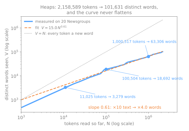
Como ler: o eixo x é o número de tokens lidos até ali e o eixo y o número de palavras distintas já vistas; os dois estão em escala log, em que uma lei de potência vira uma reta cuja inclinação é o expoente. A linha pontilhada mostra como seria a curva se todo token fosse uma palavra nova. Aqui \(\beta = 0{,}61\): dez vezes mais texto dá cerca de \(10^{0{,}61} \approx 4\) vezes mais palavras (11 mil tokens dão 3.279 palavras, 100 mil dão 18.692, um milhão dá 63.306). A curva nunca se estabiliza, porque nomes novos, erros de digitação, números e jargões continuam chegando. Um vocabulário montado hoje vai encontrar amanhã palavras que nunca viu; uma representação esparsa não tem coluna para elas.
Lei de Zipf (Zipf, 1949): a frequência cai aproximadamente como uma potência do posto.
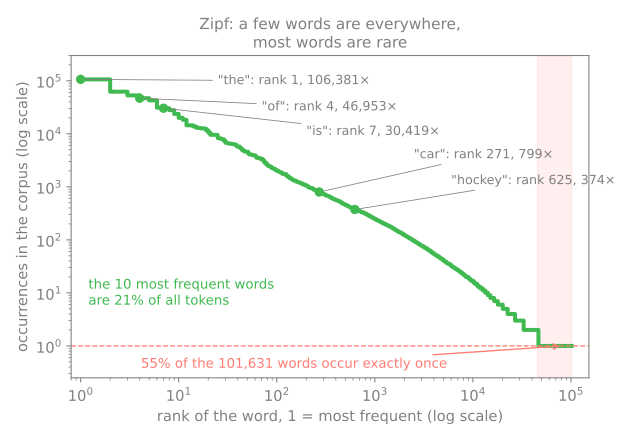
Como ler: cada ponto é uma palavra, posicionada pelo seu posto no ranking (1 = a mais frequente) no eixo x e pelo número de vezes que aparece no eixo y, os dois em escala log. No topo, "the" aparece 106.381 vezes e as 10 palavras mais frequentes somam 21% de todos os tokens; no meio, "car" (posto 271) aparece 799 vezes; na faixa vermelha, 55% das 101.631 palavras aparecem uma única vez. A maioria das colunas de uma matriz bag-of-words descreve um único documento; as poucas palavras do topo são justamente as stop words.
As duas leis já aparecem num único parágrafo. Edite o texto abaixo e mude as decisões de tokenização uma de cada vez: minúsculas, pontuação, stop words, unigramas ou bigramas. Observe o tamanho do vocabulário \(V\), a fração de termos que aparecem uma única vez e a pequena curva de Heaps à direita. O simulador corta as palavras como a regex de palavras acima: as palavras de uma letra são mantidas, então a lista de stop words tem o que remover.
Cada decisão muda o \(V\): manter maiúsculas ou pontuação acrescenta colunas; remover stop words tira as mais frequentes. Mesmo em cem palavras a maioria dos termos aparece uma única vez e, com bigramas, a curva quase segue a diagonal, porque quase todo par de vizinhos é novo.
Um mapa das abordagens
Etapa 2. Depois que o texto foi cortado em tokens, as quatro páginas desta aula transformam esses tokens em vetores de quatro jeitos diferentes, do mais simples ao mais poderoso:
| página | um documento vira | construído a partir de | o que não consegue fazer |
|---|---|---|---|
| U4.1 Bag-of-words | as contagens de suas palavras, uma coluna por palavra | contagem, sem modelo | ver a ordem das palavras, sinônimos ou palavras não vistas no fit |
| U4.2 TF-IDF | contagens pesadas pela raridade de cada palavra | contagem sobre o corpus | o mesmo: ele só muda o peso das colunas |
| U4.3 Word embeddings | um vetor denso por palavra (a média deles, para um documento) | coocorrência num corpus grande | separar os sentidos de uma mesma palavra |
| U4.4 Sentence embeddings | um vetor denso por frase ou documento curto | um transformer pré-treinado | ser barato ou explicar suas dimensões |
Bag-of-Words
A representação mais simples: um documento vira o vetor das contagens das suas palavras (uma coluna por palavra do vocabulário) e a ordem das palavras é descartada. Os três documentos acima viram uma matriz 3 × 8:
import pandas as pd

bow = CountVectorizer()
X = bow.fit_transform(docs)                        # matriz esparsa: 3 linhas, 8 colunas
print(pd.DataFrame(X.toarray(), columns=bow.get_feature_names_out(), index=['doc 1', 'doc 2', 'doc 3']))
       cachorro  comeu  do  dorme  gato  peixe  ração  sonha
doc 1         0      1   0      0     1      1      0      0
doc 2         1      1   1      0     1      0      1      0
doc 3         0      0   0      1     2      0      0      1
Cada linha é um documento, cada coluna uma palavra, cada célula uma contagem: "gato" aparece duas vezes no documento 3 ("Gato dorme, gato sonha"). Das 24 células, 13 já são zero. Os 11.314 posts dos newsgroups viram uma matriz 11.314 × 101.631 com 99,90% de zeros, guardada num formato esparso que só armazena as células não nulas. As contagens brutas são dominadas por palavras funcionais ("the" está em 9.475 dos 11.314 posts); é por isso que raramente são usadas sem peso. A página de bag-of-words monta a matriz à mão e com o CountVectorizer, compara contagem com presença (binary=True), mede o custo dos n-gramas e tem um simulador e um lab.
TF-IDF
O TF-IDF (frequência do termo × frequência inversa nos documentos) multiplica cada contagem por um peso que cai com o número de documentos que contêm a palavra. A versão do scikit-learn, para uma palavra \(t\) num documento \(d\) de um corpus de \(n\) documentos, dos quais \(\text{df}(t)\) contêm \(t\):
seguida da divisão de cada linha pelo seu comprimento. Nos três documentos acima:
from sklearn.feature_extraction.text import TfidfVectorizer

tfidf = TfidfVectorizer()
T = tfidf.fit_transform(docs)
print(pd.DataFrame([tfidf.idf_], columns=tfidf.get_feature_names_out(), index=['idf']).round(4))
print(pd.DataFrame(T.toarray(), columns=tfidf.get_feature_names_out(), index=['doc 1', 'doc 2', 'doc 3']).round(3))
     cachorro   comeu      do   dorme  gato   peixe   ração   sonha
idf    1.6931  1.2877  1.6931  1.6931   1.0  1.6931  1.6931  1.6931
       cachorro  comeu     do  dorme   gato  peixe  ração  sonha
doc 1     0.000  0.548  0.000  0.000  0.425   0.72  0.000  0.000
doc 2     0.505  0.384  0.505  0.000  0.298   0.00  0.505  0.000
doc 3     0.000  0.000  0.000  0.543  0.641   0.00  0.000  0.543
"gato", presente nos três documentos, recebe idf 1; "comeu", presente em dois, recebe 1,2877; uma palavra presente em um só recebe 1,6931. Compare o documento 1 com a sua linha na bag-of-words: as contagens eram 1, 1, 1; agora "gato" pesa 0,425 e "peixe", que só o documento 1 tem, pesa 0,720. Cada linha tem comprimento 1 e os zeros continuam onde estavam. A ideia vem de Spärck Jones (1972) e virou o padrão da recuperação de informação com Salton & Buckley (1988). A página de TF-IDF calcula cada número à mão, confere que o TfidfVectorizer concorda até a quarta casa decimal, compara documentos pela similaridade de cosseno e monta um pequeno buscador.
Similaridade e distância
Etapa 3. Quando dois textos viram vetores, "quão parecidos eles são?" vira um número calculado a partir dos dois vetores. Quatro medidas cobrem quase todos os usos:
- similaridade de cosseno: compara as direções dos dois vetores e ignora os seus comprimentos. 1 significa que eles apontam para o mesmo lado (as mesmas palavras nas mesmas proporções); 0 significa que não têm nada em comum; com contagens, ela nunca é negativa. É a medida usada em toda esta aula;
- distância euclidiana: a distância em linha reta entre os dois pontos, a que o k-means usa. 0 significa vetores idênticos; ela cresce com qualquer diferença, inclusive de comprimento;
- produto escalar: multiplique os dois vetores coordenada a coordenada e some. Ele é grande quando os dois têm valores grandes nas mesmas colunas; por isso cresce com o tamanho dos documentos;
- similaridade de Jaccard: esqueça as contagens e compare os dois conjuntos de tokens: o número de tokens em comum dividido pelo número de tokens distintos nos dois. 1 significa o mesmo conjunto de palavras; 0, nenhuma palavra em comum.
Pegue o documento 1 da bag-of-words, o documento 3 e um terceiro documento que é o documento 1 escrito três vezes: o mesmo conteúdo, três vezes mais longo:
from sklearn.metrics import jaccard_score
from sklearn.metrics.pairwise import cosine_similarity, euclidean_distances

A, B, A3 = bow.transform(["O gato comeu o peixe.",
                          "Gato dorme, gato sonha.",
                          "O gato comeu o peixe. " * 3]).toarray()    # A3: o documento A três vezes
print('columns:', list(bow.get_feature_names_out()))
print('A  =', A, ' B =', B, ' A3 =', A3)
for name, u, v in [('A and B ', A, B), ('A and A3', A, A3), ('B and A3', B, A3)]:
    print(f"{name}  cosine {cosine_similarity([u], [v])[0, 0]:.3f} · Euclidean {euclidean_distances([u], [v])[0, 0]:.3f}"
          f" · dot {u @ v:2d} · Jaccard {jaccard_score(u > 0, v > 0):.3f}")
columns: ['cachorro', 'comeu', 'do', 'dorme', 'gato', 'peixe', 'ração', 'sonha']
A  = [0 1 0 0 1 1 0 0]  B = [0 0 0 1 2 0 0 1]  A3 = [0 3 0 0 3 3 0 0]
A and B   cosine 0.471 · Euclidean 2.236 · dot  2 · Jaccard 0.200
A and A3  cosine 1.000 · Euclidean 3.464 · dot  9 · Jaccard 1.000
B and A3  cosine 0.471 · Euclidean 4.583 · dot  6 · Jaccard 0.200
Leia como um problema de busca: a consulta é A; os candidatos são B (outro assunto, que só tem "gato" em comum) e A3 (exatamente o mesmo assunto, só que mais longo).
- o cosseno diz o que queremos: A3 é idêntico a A (1,000) e B é uma correspondência parcial (0,471). B contra A3 também recebe 0,471, o mesmo que B contra A: repetir um documento não muda a sua direção;
- a distância euclidiana inverte a resposta: A3 fica mais longe de A (3,464) do que B (2,236), só porque A3 é mais longo;
- o produto escalar cresce com o comprimento: B contra A3 marca 6, o triplo do seu escore contra A, para o mesmo conteúdo;
- o Jaccard concorda com o cosseno aqui (1,000 e 0,200) porque só olha quais palavras estão presentes, o que também o deixa cego a quantas vezes elas aparecem.
É por isso que o cosseno é o padrão para texto: documentos têm todos os tamanhos; o tamanho de um documento diz pouco sobre o seu assunto. Quando os vetores são antes escalados para comprimento 1, as três medidas concordam: o produto escalar é o cosseno e a distância euclidiana ordena todos os pares na ordem inversa do cosseno. As linhas do TF-IDF já têm comprimento 1 (o scikit-learn divide cada linha pelo seu comprimento) e os sentence embeddings costumam ser pedidos com normalize_embeddings=True; na prática, eles são comparados por um produto escalar.
Os limites das representações esparsas
No bag-of-words e no TF-IDF, cada palavra é um eixo próprio, ortogonal a todas as outras. A página de TF-IDF mede as consequências em pares de frases:
- sinônimos dão zero: "o carro é rápido" e "o automóvel é veloz" têm cosseno 0,00;
- a ordem das palavras é invisível: "o cachorro mordeu o homem" e "o homem mordeu o cachorro" têm cosseno 1,00;
- uma grafia, dois sentidos: manga (da camisa ou a fruta) faz duas frases sem relação parecerem próximas, enquanto duas frases de mesmo sentido e palavras diferentes parecem não ter relação (0,14 nos dois casos);
- palavras novas somem: uma palavra não vista no
fitnão tem coluna, então uma frase feita só de palavras novas vira o vetor nulo.
No lab de TF-IDF, os 10 melhores resultados para "image" e os 10 melhores para "picture" não têm nenhum post em comum. São essas falhas que motivaram as representações densas.
Embeddings densos
De volta à etapa 2, agora para a família densa.
"Você conhecerá uma palavra pelas companhias que ela mantém" (Firth, 1957). A hipótese distribucional (Harris, 1954) diz que palavras usadas em contextos parecidos têm significados parecidos: "carro" e "automóvel" raramente aparecem na mesma frase, mas aparecem ao lado das mesmas palavras (motor, concessionária, pneu). As representações densas exploram isso. Em vez de uma coluna por palavra, cada palavra ou texto recebe um vetor de algumas centenas de números, aprendido num corpus grande de modo que contextos parecidos deem vetores próximos. Nenhum número isolado significa algo; só as distâncias entre vetores significam.
Word embeddings
O word2vec (Mikolov et al., 2013) aprende um vetor por palavra treinando uma rede pequena para prever as palavras em volta de cada palavra; o GloVe (Pennington et al., 2014) chega a vetores parecidos fatorando uma tabela de contagens de coocorrência. Sinônimos ficam próximos e algumas direções do espaço codificam relações. A limitação é um vetor por palavra, qualquer que seja o sentido. A página de word embeddings mostra como esses vetores são aprendidos e o que eles capturam.
Como é um desses vetores: os vetores GloVe pré-treinados, treinados em 6 bilhões de tokens de notícias e da Wikipédia em inglês, na sua menor versão (400.000 palavras, 50 números cada). São vetores do inglês, então os exemplos são palavras em inglês:
import gensim.downloader as api                   # pip install gensim

glove = api.load('glove-wiki-gigaword-50')        # ~66 MB, baixado uma vez
print('cat =', glove['cat'][:8].round(3), '... (50 numbers, none of them zero)')
print('nearest to cat:', ', '.join(f"{w} {c:.2f}" for w, c in glove.most_similar('cat', topn=5)))
for a, b in [('car', 'automobile'), ('car', 'banana')]:
    print(f"cosine {a} / {b}: {glove.similarity(a, b):.2f}")
cat = [ 0.453 -0.501 -0.537 -0.016  0.222  0.546 -0.673 -0.689] ... (50 numbers, none of them zero)
nearest to cat: dog 0.92, rabbit 0.85, monkey 0.80, rat 0.79, cats 0.79
cosine car / automobile: 0.70
cosine car / banana: 0.22
Os 50 números de "cat" (gato) não significam nada um a um; o que carrega o sentido é quais vetores estão por perto, medido pelo cosseno: as palavras mais próximas de "cat" são outros animais, a começar por "dog" (cachorro, 0,92). "car" e "automobile", que nunca dividiram uma coluna na bag-of-words, agora têm cosseno 0,70, contra 0,22 de "car" e "banana".
Sentence embeddings: contextuais e de documento inteiro
Modelos transformer como o BERT (Devlin et al., 2019) calculam o vetor de cada token a partir da frase inteira em volta dele, então manga recebe um vetor diferente ao lado de "camisa" e ao lado de "madura". O Sentence-BERT (Reimers & Gurevych, 2019) treina um modelo assim para que um único vetor resuma uma frase ou um documento curto inteiro e para que o cosseno entre dois desses vetores acompanhe a proximidade dos seus significados. A biblioteca sentence-transformers empacota centenas desses modelos, vários deles multilíngues. A página de sentence embeddings mostra como eles são construídos e como usá-los; o resto desta página usa um deles.
É um modelo multilíngue pequeno do sentence-transformers (a página de sentence embeddings o explica): cada texto vira 384 números; textos em mais de 50 línguas compartilham o mesmo espaço. Carregá-lo baixa cerca de 470 MB na primeira vez.
# pip install sentence-transformers
from sentence_transformers import SentenceTransformer

model = SentenceTransformer('paraphrase-multilingual-MiniLM-L12-v2')
emb = model.encode(["o carro é rápido",
                    "o automóvel é veloz",       # o mesmo sentido, nenhuma palavra em comum
                    "a taxa de juros subiu"],    # sem relação
                   normalize_embeddings=True)
print(emb.shape)
print('o carro é rápido =', emb[0][:8].round(3), '... (384 numbers)')
for j in [1, 2]:
    print(f"vs {j}: cosine {cosine_similarity(emb[[0]], emb[[j]])[0, 0]:.2f} · dot {emb[0] @ emb[j]:.2f}"
          f" · Euclidean {euclidean_distances(emb[[0]], emb[[j]])[0, 0]:.2f}")
(3, 384)
o carro é rápido = [ 0.016  0.033 -0.08   0.037 -0.014 -0.002  0.039 -0.028] ... (384 numbers)
vs 1: cosine 0.97 · dot 0.97 · Euclidean 0.25
vs 2: cosine 0.23 · dot 0.23 · Euclidean 1.24
Uma frase inteira vira 384 números, qualquer que seja o seu tamanho. A paráfrase, sem nenhuma palavra em comum, recebe cosseno 0,97; a frase sem relação, 0,23. Como os vetores foram escalados para comprimento 1 (normalize_embeddings=True), o produto escalar é igual ao cosseno e a distância euclidiana conta a mesma história ao contrário: pequena para a paráfrase, grande para o par sem relação.
Representações esparsas vs densas
As duas famílias produzem vetores de formatos muito diferentes. Pegue uma frase em inglês (para que as três representações consigam lê-la) e represente-a de três jeitos: uma bag-of-words sobre o vocabulário dos 11.314 posts dos newsgroups, a média dos vetores GloVe das suas palavras e o sentence embedding:
import numpy as np

s_en = "the cat sleeps on the couch"
bow_news = CountVectorizer().fit(news.data)                  # as 101.631 palavras dos newsgroups
x = bow_news.transform([s_en])
vocab = bow_news.get_feature_names_out()
print(f"bag-of-words   length {x.shape[1]:>7,} · non-zero {x.nnz:>3}:",
      ', '.join(f"{vocab[j]} (column {j:,}) = {v}" for j, v in zip(x.indices, x.data)), '· all others 0')
g = np.mean([glove[w] for w in s_en.split()], axis=0)        # média dos 6 vetores de palavras
print(f"GloVe average  length {g.size:>7,} · non-zero {np.count_nonzero(g):>3}:", g[:6].round(3), '...')
e = model.encode(s_en)
print(f"sentence emb.  length {e.size:>7,} · non-zero {np.count_nonzero(e):>3}:", e[:6].round(3), '...')
bag-of-words   length 101,631 · non-zero   5: cat (column 26,019) = 1, couch (column 30,064) = 1, on (column 68,080) = 1, sleeps (column 83,252) = 1, the (column 88,532) = 2 · all others 0
GloVe average  length      50 · non-zero  50: [ 0.271  0.037 -0.335 -0.147  0.541  0.055] ...
sentence emb.  length     384 · non-zero 384: [ 0.39  -0.348 -0.135  0.145  0.115  0.278] ...
| esparsa (bag-of-words, TF-IDF) | densa (word e sentence embeddings) | |
|---|---|---|
| comprimento | uma coluna por palavra do vocabulário: aqui, 101.631 | fixado pelo modelo: 50 neste GloVe, 384 neste modelo de frases |
| valores não nulos | só as palavras do texto: aqui, 5 | todos |
| o que uma coordenada significa | legível: a coluna 26.019 é "quantas vezes cat aparece" | nada sozinha; só as distâncias entre vetores significam algo |
| como é guardada | só as células não nulas (índice, valor) | um vetor comum de números reais |
| dois textos sem palavra em comum | nenhuma coluna não nula em comum: cosseno 0 | ainda podem ficar próximos |
Esparso quer dizer que quase toda coordenada é zero e que as poucas não nulas são legíveis: cada uma é uma palavra do texto. Denso quer dizer que toda coordenada tem um valor (nenhum legível sozinho) e que a informação mora na geometria. Essa é toda a diferença entre as duas metades desta aula e ela decide tudo o que vem depois: vetores esparsos só aproximam textos que dividem palavras; vetores densos aproximam textos que dividem sentido.
Agora compare as quatro técnicas você mesmo. Escolha duas frases ou um dos pares prontos e observe os dois vetores em cada representação (as faixas da bag-of-words e do TF-IDF quase vazias, as densas cheias), além do cosseno, da distância euclidiana e do produto escalar de cada uma. Comece pela paráfrase (nenhuma palavra em comum), depois a ordem das palavras, depois a palavra ambígua banco (o banco que sobe os juros, o banco da praça) contra o par de mesmo sentido em outras palavras; por fim, marque B três vezes e comprimento 1 e veja quais números mudam. Os vetores GloVe só existem para o inglês; com as frases em português, essa faixa usa a frase em inglês do mesmo item.
Na paráfrase, as duas representações esparsas dão cosseno 0 e as duas densas não. Com a ordem trocada, bag-of-words, TF-IDF e média GloVe ficam idênticos, porque nenhum deles vê a ordem; só o sentence embedding se mexe, mas pouco. Repetir B muda a distância euclidiana e o produto escalar da bag-of-words, mas não o seu cosseno; com comprimento 1, o produto escalar e o cosseno viram o mesmo número.
Esparso vs denso: quando usar cada um
Etapa 4. Tudo nesta seção é medido com o modelo multilíngue carregado acima, contra o TF-IDF do scikit-learn.
Similaridade: os mesmos pares, dos dois jeitos
Os pares da seção de limites e mais alguns. O TF-IDF é ajustado em todas as frases da tabela:
pairs_all = [("o carro é rápido", "o automóvel é veloz"),
             ("comprei um celular novo", "adquiri um smartphone novo"),
             ("o gato dorme no sofá", "the cat sleeps on the couch"),
             ("a manga da camisa rasgou", "o punho da blusa descosturou"),
             ("a manga da camisa rasgou", "comi uma manga madura"),
             ("o filme é muito bom", "o filme não é bom"),
             ("o cachorro mordeu o homem", "o homem mordeu o cachorro"),
             ("a taxa de juros subiu", "o time venceu o jogo")]
sentences = list(dict.fromkeys(s for p in pairs_all for s in p))   # sem repetição, na ordem
tf_pairs = TfidfVectorizer().fit(sentences)
rows = []
for a, b in pairs_all:
    e = model.encode([a, b], normalize_embeddings=True)
    rows.append({'A': a, 'B': b,
                 'TF-IDF': cosine_similarity(tf_pairs.transform([a, b]))[0, 1],
                 'embedding': e[0] @ e[1]})
print(pd.DataFrame(rows).round(2).to_string(index=False))
                        A                            B  TF-IDF  embedding
         o carro é rápido          o automóvel é veloz    0.00       0.97
  comprei um celular novo   adquiri um smartphone novo    0.43       0.91
     o gato dorme no sofá  the cat sleeps on the couch    0.00       0.98
 a manga da camisa rasgou o punho da blusa descosturou    0.21       0.87
 a manga da camisa rasgou        comi uma manga madura    0.21       0.35
      o filme é muito bom            o filme não é bom    0.60       0.46
o cachorro mordeu o homem    o homem mordeu o cachorro    1.00       0.98
    a taxa de juros subiu         o time venceu o jogo    0.00       0.14
Linha a linha:
- paráfrases ("comprei um celular novo" / "adquiri um smartphone novo"): 0,91 contra 0,43; o TF-IDF só enxerga "um" e "novo";
- tradução (linha 3): a frase em português e sua tradução para o inglês não têm nenhum token em comum, mas o modelo multilíngue as coloca em 0,98. Uma consulta em português pode recuperar documentos escritos em inglês;
- as duas linhas de "manga": o TF-IDF dá o mesmo 0,21 aos dois pares, enquanto o embedding separa o par manga-e-punho (0,87) do par manga-e-fruta (0,35);
- negação ("o filme é muito bom" / "o filme não é bom"): o embedding fica abaixo do TF-IDF (0,46 contra 0,60), mas longe de "oposto". Duas frases sobre o quanto o mesmo filme é bom se sobrepõem bastante em significado;
- ordem das palavras: 0,98. Os sentence embeddings também confundem quem mordeu quem;
- frases sem relação dão 0,14, não 0. Os cossenos de embeddings ocupam uma escala comprimida: o que carrega a informação é a ordenação (0,97 contra 0,14), não o valor absoluto. Um limiar ajustado para um modelo não vale para outro.
Tokens raros e exatos: onde o TF-IDF é mais forte
Considere duas entradas de uma central de ajuda que só diferem pelo código de erro, com uma consulta para cada código:
entries = ["O que fazer quando aparece o erro 0x80070005 na instalação?",
           "O que fazer quando aparece o erro 0x80004005 na atualização?"]
tf_entries = TfidfVectorizer().fit(entries)
E_entries = model.encode(entries, normalize_embeddings=True)
for q in ["erro 0x80070005", "erro 0x80004005"]:
    t = cosine_similarity(tf_entries.transform([q]), tf_entries.transform(entries))[0]
    e = E_entries @ model.encode(q, normalize_embeddings=True)
    print(f"{q}:  TF-IDF {t.round(2)}   embedding {e.round(2)}")
erro 0x80070005:  TF-IDF [0.55 0.18]   embedding [0.8  0.77]
erro 0x80004005:  TF-IDF [0.18 0.55]   embedding [0.81 0.78]
As duas representações põem a entrada certa em primeiro lugar, mas observe as margens. Para o TF-IDF, o código é o token mais distintivo de cada entrada e decide a correspondência, 0,55 contra 0,18. Para o embedding, as duas entradas são "uma mensagem de erro na instalação ou atualização"; o código altera o escore em só 0,03 (0,80 contra 0,77). Com centenas de códigos parecidos, nomes de produtos ou referências a leis, a correspondência exata é o que você quer; sistemas de busca em produção costumam combinar as duas ordenações (busca híbrida).
Classificação: quantos rótulos você tem?
Quase todo projeto acaba precisando de uma previsão (encaminhar um chamado, etiquetar um post); a representação vira, então, a entrada de um modelo supervisionado. Nenhum foi ensinado ainda, então usamos uma regressão logística como caixa-preta (ela tem sua própria aula mais adiante): ela recebe um vetor e um rótulo para cada post de treino e aprende a prever os rótulos de posts novos. Só a representação muda.
Quatro newsgroups da coleção 20 Newsgroups (carros, medicina, espaço, armas), com a divisão oficial do scikit-learn: o modelo aprende com os posts mais antigos e é avaliado nos mais recentes, um hold-out que ele nunca vê durante o treino. Para ver quanto dado rotulado cada representação precisa, treinamos com 5, 10, 25 e 100 posts rotulados por classe e, depois, com todos:
from sklearn.datasets import fetch_20newsgroups
from sklearn.linear_model import LogisticRegression

def load(subset, cats):
    d = fetch_20newsgroups(subset=subset, categories=cats,
                           remove=('headers', 'footers', 'quotes'), random_state=0)
    keep = [i for i, t in enumerate(d.data) if len(t.split()) >= 20]   # descarta posts vazios ou muito curtos
    return [d.data[i] for i in keep], d.target[keep]

cats = ['rec.autos', 'sci.med', 'sci.space', 'talk.politics.guns']
docs_tr, y_tr = load('train', cats)       # posts mais antigos
docs_te, y_te = load('test', cats)        # posts mais recentes: o hold-out
E_tr = model.encode(docs_tr, normalize_embeddings=True)
E_te = model.encode(docs_te, normalize_embeddings=True)
print(len(docs_tr), 'training posts ·', len(docs_te), 'test posts')

rng = np.random.default_rng(0)
print('labeled posts per class | TF-IDF + clf | embedding + clf')
for n in [5, 10, 25, 100, 'all']:
    if n == 'all':
        idx = np.arange(len(docs_tr))
    else:
        idx = np.concatenate([rng.choice(np.flatnonzero(y_tr == c), n, replace=False) for c in range(4)])
    vec = TfidfVectorizer(stop_words='english').fit([docs_tr[i] for i in idx])
    sparse_clf = LogisticRegression(max_iter=2000).fit(vec.transform([docs_tr[i] for i in idx]), y_tr[idx])
    dense_clf = LogisticRegression(max_iter=2000).fit(E_tr[idx], y_tr[idx])
    print(f"{str(n):>23s} | {sparse_clf.score(vec.transform(docs_te), y_te):11.3f} | "
          f"{dense_clf.score(E_te, y_te):15.3f}")
2097 training posts · 1364 test posts
labeled posts per class | TF-IDF + clf | embedding + clf
                      5 |       0.557 |           0.819
                     10 |       0.601 |           0.851
                     25 |       0.725 |           0.886
                    100 |       0.850 |           0.897
                    all |       0.904 |           0.901
O escore é a acurácia nos 1.364 posts de teste; chutar sempre uma classe daria cerca de 25%. Com 5 posts rotulados por classe, o classificador sobre embeddings chega a 81,9% e o sobre TF-IDF a 55,7%. Com 20 posts de treino no total, o TF-IDF viu só algumas centenas de palavras distintas; um post de teste que por acaso não use nenhuma delas vira um vetor nulo. O modelo de embeddings já chega sabendo que "sedan" fica perto de "car", pelo texto em que foi treinado. À medida que os rótulos se acumulam, o TF-IDF aprende o vocabulário de cada classe a partir dos próprios dados; com todos os 2.097 posts, os dois empatam: 90,4% contra 90,1%.
O que os escores não mostram é o custo. No notebook usado para escrever esta página, o TfidfVectorizer processa os 2.097 posts de treino em 0,2 segundo, enquanto o modelo de embeddings precisa de cerca de um minuto na mesma CPU (10 segundos na GPU do notebook), depois de baixar 470 MB.
| Esparso (bag-of-words, TF-IDF) | Denso (sentence embeddings) | |
|---|---|---|
| tamanho do vetor de um documento | \(\lvert V \rvert\) colunas (10⁴–10⁶), 99,9% de zeros | 384–1.024 números, nenhum nulo |
| sinônimos, paráfrases | ortogonais: cosseno 0,00 | próximos: cosseno 0,97 |
palavras nunca vistas no fit | descartadas | tratadas (pedaços de subpalavras) |
| tokens raros e exatos (códigos, nomes, jargão) | idf alto, sinal forte | diluídos no sentido geral |
| outras línguas | vocabulários separados | espaço compartilhado com um modelo multilíngue |
| poucos exemplos rotulados (5 por classe, acima) | 55,7% | 81,9% |
| muitos exemplos rotulados (os 2.097, acima) | 90,4% | 90,1% |
| interpretabilidade | cada coluna é uma palavra | colunas abstratas |
| custo | frações de segundo numa CPU, sem modelo | um modelo pré-treinado; uma GPU ajuda |
| usos típicos | busca por palavras-chave, baselines lineares fortes, jargão de domínio | busca semântica, poucos rótulos, agrupamento, BERTopic |
Na prática: comece pelo TF-IDF, que é barato e difícil de bater quando há muitos dados rotulados e vocabulário de domínio; recorra aos embeddings quando o significado importa mais que as palavras exatas (busca, textos curtos, paráfrases, várias línguas) ou quando os rótulos são escassos; e quando tanto os tokens exatos quanto o significado importam, combine os dois.
Para onde isso leva
Modelagem de Tópicos & BERTopic usa as duas metades desta aula. Ela gera embeddings dos documentos com um sentence-transformer, reduz os vetores com UMAP, agrupa-os com HDBSCAN e depois descreve cada grupo com uma variante do TF-IDF calculada por agrupamento. Esse pipeline é o BERTopic.
Exercícios
- Com o ajuste de Heaps desta página (\(V = 15{,}0\,N^{0{,}61}\)), quantas palavras distintas você esperaria num corpus dez vezes maior (cerca de 21,6 milhões de tokens)? O que isso implica para um vocabulário ajustado hoje e usado por um ano?
- Tokenize "Não gostei do filme, não!" com o analisador padrão do scikit-learn, com a lista mínima de stop words desta página e com
ngram_range=(1, 2). Qual versão mantém a negação? - Para cada tarefa, escolha esparso ou denso e justifique numa frase: (a) achar o contrato que cita a "Lei 13.709/2018"; (b) agrupar 50.000 avaliações de clientes por assunto; (c) classificar 300 chamados de suporte em 5 filas, com 20 exemplos rotulados; (d) buscar artigos em inglês com consultas em português.
Lab: esparso vs denso em posts reais
Quatro newsgroups da coleção 20 Newsgroups (computação gráfica, beisebol, eletrônica e cristianismo), cerca de 2.100 posts, representados duas vezes: com TF-IDF e com sentence embeddings. O lab coloca os dois lado a lado nas tarefas desta página: achar posts sobre o mesmo assunto, responder consultas de busca, desenhar um mapa e alimentar um classificador caixa-preta com muitos e com poucos rótulos. Os labs de bag-of-words e de TF-IDF olham por dentro da representação esparsa dos mesmos posts.
O lab roda em cerca de dois minutos numa CPU; o passo 2, que codifica cada post com uma rede neural, é quase todo esse tempo (um ambiente com GPU no Colab faz isso em poucos segundos). Rode os blocos em ordem, numa mesma sessão. Para trabalhar direto nele, baixe o notebook do lab e abra no Jupyter ou no Colab (Arquivo → Fazer upload de notebook).
Passo 1 — carregar os posts
# No Colab, rode uma vez:  !pip install sentence-transformers
import numpy as np
import pandas as pd
from sklearn.datasets import fetch_20newsgroups

cats = ['comp.graphics', 'rec.sport.baseball', 'sci.electronics', 'soc.religion.christian']
raw = fetch_20newsgroups(subset='train', categories=cats,
                         remove=('headers', 'footers', 'quotes'), random_state=0)
keep = [i for i, t in enumerate(raw.data) if len(t.split()) >= 20]   # descarta posts vazios ou muito curtos
docs = [raw.data[i] for i in keep]
y = raw.target[keep]
names = np.array(raw.target_names)
print(len(docs), 'posts:', ', '.join(f"{g} {c}" for g, c in zip(names, np.bincount(y))))
print(f"words per post: median {np.median([len(d.split()) for d in docs]):.0f}")
2116 posts: comp.graphics 521, rec.sport.baseball 495, sci.electronics 535, soc.religion.christian 565
words per post: median 97
Os mesmos 2.116 posts dos labs de bag-of-words e de TF-IDF: quatro grupos equilibrados, sem cabeçalhos, assinaturas ou respostas citadas. Os posts com menos de 20 palavras foram descartados. Um post mediano tem 97 palavras.
Passo 2 — duas representações dos mesmos posts
from sentence_transformers import SentenceTransformer
from sklearn.feature_extraction.text import TfidfVectorizer

tfidf = TfidfVectorizer(stop_words='english', min_df=2)
T = tfidf.fit_transform(docs)
sparse_mb = (T.data.nbytes + T.indices.nbytes + T.indptr.nbytes) / 1e6
print(f"TF-IDF:     {T.shape}, {T.nnz / T.shape[0]:.0f} non-zeros per post, {sparse_mb:.1f} MB")

model = SentenceTransformer('all-MiniLM-L6-v2')      # inglês, 384 dimensões, ~90 MB
E = model.encode(docs, batch_size=64, normalize_embeddings=True)
print(f"embeddings: {E.shape}, all non-zero, {E.nbytes / 1e6:.1f} MB · reads at most {model.max_seq_length} tokens per post")
TF-IDF:     (2116, 12001), 58 non-zeros per post, 1.5 MB
embeddings: (2116, 384), all non-zero, 3.3 MB · reads at most 256 tokens per post
Como ler:
- TF-IDF: 12.001 colunas, mas um post preenche em média só 58 delas; guardada em formato esparso, a matriz inteira ocupa 1,5 MB.
- Embeddings: 384 colunas, nenhuma nula, 3,3 MB em floats de 32 bits. Menos colunas, mas mais memória que a matriz esparsa aqui, porque nada é zero.
- 256 tokens: este modelo lê só o começo de cada post; o resto de um post mais longo é ignorado. O modelo multilíngue da página lê 128.
O tempo vai todo na codificação: o TF-IDF é uma passada de contagem; os embeddings, uma passada de uma rede de 6 camadas por post.
Passo 3 — qual das duas acha posts sobre o mesmo assunto?
from sklearn.feature_extraction.text import CountVectorizer
from sklearn.neighbors import NearestNeighbors

def agreement(V, k=5):
    """Fração dos k posts mais próximos (cosseno) de cada post que vêm do mesmo newsgroup."""
    nn = NearestNeighbors(n_neighbors=k + 1, metric='cosine').fit(V)
    _, idx = nn.kneighbors(V)
    return (y[idx[:, 1:]] == y[:, None]).mean()

print(f"chance level:            {np.sum(np.bincount(y) ** 2) / len(y) ** 2:.3f}")
print(f"raw counts:              {agreement(CountVectorizer().fit_transform(docs)):.3f}")
print(f"TF-IDF:                  {agreement(T):.3f}")
print(f"sentence embeddings:     {agreement(E):.3f}")
A concordância de vizinhos dos labs das subpáginas: para cada post, a fração dos seus 5 posts mais próximos (cosseno) que vêm do mesmo newsgroup; 0,251 por acaso. As contagens brutas chegam a 0,490, o TF-IDF a 0,850 e os sentence embeddings a 0,948. O modelo de embeddings nunca viu estes newsgroups nem seus rótulos: ele chega com uma noção de quais textos falam de coisas parecidas, aprendida no texto em que foi treinado. Essa noção coincide bem com os newsgroups.
Passo 4 — busca semântica contra busca por palavras-chave
from sklearn.metrics.pairwise import cosine_similarity

queries = {"my picture looks blurry after I enlarge it": 'comp.graphics',
           "software to convert a photo from one file format to another": 'comp.graphics',
           "the umpire made a terrible call last night": 'rec.sport.baseball',
           "why does my TV screen flicker": 'sci.electronics',
           "how to stop my circuit from overheating": 'sci.electronics',
           "does the soul survive after death": 'soc.religion.christian'}
T_q = tfidf.transform(list(queries))
E_q = model.encode(list(queries), normalize_embeddings=True)
hits = np.zeros(2, dtype=int)
for (q, group), tq, eq in zip(queries.items(), T_q, E_q):
    top_s = np.argsort(-cosine_similarity(tq, T).ravel())[:5]       # os 5 melhores posts, TF-IDF
    top_d = np.argsort(-(E @ eq))[:5]                                # os 5 melhores posts, embeddings
    h = np.sum(names[y[top_s]] == group), np.sum(names[y[top_d]] == group)
    hits += h
    print(f"{q:60s} TF-IDF {h[0]}/5 · embedding {h[1]}/5")
print(f"{'total':60s} TF-IDF {hits[0]}/30 · embedding {hits[1]}/30")
print('best embedding hit for the last query:', ' '.join(docs[top_d[0]].split())[:100])
my picture looks blurry after I enlarge it                   TF-IDF 3/5 · embedding 5/5
software to convert a photo from one file format to another  TF-IDF 5/5 · embedding 5/5
the umpire made a terrible call last night                   TF-IDF 3/5 · embedding 5/5
why does my TV screen flicker                                TF-IDF 3/5 · embedding 5/5
how to stop my circuit from overheating                      TF-IDF 5/5 · embedding 5/5
does the soul survive after death                            TF-IDF 2/5 · embedding 5/5
total                                                        TF-IDF 21/30 · embedding 30/30
best embedding hit for the last query: Now this is getting interesting! I was raised Roman Catholic before becoming an atheist, so I have s
Cada consulta foi escrita à mão para um dos quatro grupos; contamos quantos dos 5 posts recuperados vêm desse grupo: 30 de 30 para os embeddings, 21 de 30 para o TF-IDF. O TF-IDF acerta os 5 quando a consulta usa as palavras do próprio grupo ("convert", "file", "format"; "circuit") e cai para 2 ou 3 quando descreve o assunto com outras palavras ou usa palavras fora do seu vocabulário ("flicker"). O melhor resultado dos embeddings para "does the soul survive after death" é um post que pergunta onde a alma fica entre a morte e a ressurreição: exatamente o assunto da consulta.
Passo 5 — olhar os dois espaços
import matplotlib.pyplot as plt
from sklearn.decomposition import TruncatedSVD
from sklearn.manifold import TSNE
from sklearn.metrics import silhouette_score

T50 = TruncatedSVD(n_components=50, random_state=0).fit_transform(T)
maps = {'TF-IDF (SVD to 50-d)': TSNE(2, init='pca', random_state=0).fit_transform(T50),
        'sentence embeddings': TSNE(2, init='pca', random_state=0).fit_transform(E)}

fig, axes = plt.subplots(1, 2, figsize=(11, 4.5))
for ax, (title, P) in zip(axes, maps.items()):
    for c in range(4):
        ax.scatter(P[y == c, 0], P[y == c, 1], s=4, label=names[c])
    ax.set_title(title)
axes[1].legend(markerscale=3)
plt.show()

print(f"silhouette of the newsgroups, TF-IDF space:    {silhouette_score(T, y, metric='cosine'):.3f}")
print(f"silhouette of the newsgroups, embedding space: {silhouette_score(E, y, metric='cosine'):.3f}")
silhouette of the newsgroups, TF-IDF space:    0.012
silhouette of the newsgroups, embedding space: 0.120
Os dois mapas são feitos do mesmo jeito (t-SNE, com o newsgroup usado só para colorir). Com embeddings, os quatro grupos formam quatro ilhas separadas, com gráficos e eletrônica, os dois grupos técnicos, lado a lado. Com TF-IDF, religião e beisebol se separam, mas eletrônica se espalha pelo meio e se sobrepõe a gráficos. A silhueta (da aula de agrupamento), calculada no espaço completo com o newsgroup como rótulo de grupo, quantifica isso: 0,012 para o TF-IDF, 0,120 para os embeddings. As duas são baixas, porque em centenas de dimensões os grupos se sobrepõem e todo post de fronteira pesa contra, mas o espaço dos embeddings é dez vezes mais organizado por assunto.
Passo 6 — o mesmo classificador caixa-preta nas duas representações
from sklearn.linear_model import LogisticRegression
from sklearn.model_selection import train_test_split

idx_tr, idx_te = train_test_split(np.arange(len(docs)), test_size=0.3, stratify=y, random_state=0)
docs_tr = [docs[k] for k in idx_tr]
docs_te = [docs[k] for k in idx_te]

vec = TfidfVectorizer(stop_words='english', min_df=2).fit(docs_tr)     # ajustado só nos posts de treino
X_tr, X_te = vec.transform(docs_tr), vec.transform(docs_te)
clf = LogisticRegression(max_iter=2000)                                 # uma caixa-preta, por enquanto

print(f"TF-IDF     + classifier: {clf.fit(X_tr, y[idx_tr]).score(X_te, y[idx_te]):.3f}")
print(f"embeddings + classifier: {clf.fit(E[idx_tr], y[idx_tr]).score(E[idx_te], y[idx_te]):.3f}")

rng = np.random.default_rng(0)
few = np.concatenate([rng.choice(idx_tr[y[idx_tr] == c], 10, replace=False) for c in range(4)])
vec_few = TfidfVectorizer(stop_words='english').fit([docs[k] for k in few])
acc_s = clf.fit(vec_few.transform([docs[k] for k in few]), y[few]).score(vec_few.transform(docs_te), y[idx_te])
acc_d = clf.fit(E[few], y[few]).score(E[idx_te], y[idx_te])
print(f"only 10 labeled posts per class: TF-IDF {acc_s:.3f} · embeddings {acc_d:.3f}")
TF-IDF     + classifier: 0.917
embeddings + classifier: 0.951
only 10 labeled posts per class: TF-IDF 0.702 · embeddings 0.910
A caixa-preta é de novo uma regressão logística. A divisão separa 30% dos posts (635) como hold-out, estratificado por grupo; o vocabulário do TF-IDF é ajustado só nos posts de treino. Com os 1.481 posts de treino, os embeddings ganham por 3,4 pontos, 95,1% contra 91,7%. Com 10 posts rotulados por classe, 40 no total, eles mantêm 91,0% enquanto o TF-IDF cai para 70,2%. Nos quatro newsgroups da página, o TF-IDF tinha alcançado os embeddings com 2.097 rótulos; aqui os embeddings continuam na frente mesmo com todos. Qual representação vence com muitos rótulos depende do corpus; com poucos rótulos, o modelo pré-treinado leva grande vantagem.
Sua vez
- Busca entre línguas. Troque o modelo do passo 2 por
paraphrase-multilingual-MiniLM-L12-v2e busque nos posts em inglês com as consultas do passo 4 traduzidas para o português ("minha foto fica borrada quando eu amplio", ...). Quantos dos 30 resultados são do grupo certo? Depois tente as consultas em português com o TF-IDF. - Busca híbrida. Para cada consulta do passo 4, ordene os posts por \(0{,}5 \cdot \cos_{\text{TF-IDF}} + 0{,}5 \cdot \cos_{\text{embedding}}\). A combinação chega a vencer os embeddings sozinhos? Escreva uma consulta em que o TF-IDF deveria vencer (um nome de produto raro que aparece em poucos posts) e teste.
- Quão poucos rótulos? Transforme a última parte do passo 6 num laço sobre 2, 5, 10, 25 e 50 posts rotulados por classe, com 5 sementes diferentes para cada um. Depois, plote a acurácia média das duas representações contra o número de rótulos. Onde as curvas se encontram, se é que se encontram?
- Posts longos. O
all-MiniLM-L6-v2lê só os primeiros 256 tokens de cada post. Divida cada post em pedaços de cerca de 150 palavras, gere os embeddings dos pedaços e represente o post pela média dos vetores dos pedaços. A concordância de vizinhos do passo 3 muda?
Material de aula
Notebook do lab
O lab desta página como notebook, pronto para o Jupyter ou o Colab: notebook do lab. No Colab, rode !pip install sentence-transformers na primeira célula. As quatro subpáginas têm seus próprios labs: bag-of-words, TF-IDF, word embeddings e sentence embeddings.
Referências
- Harris, Z. S. "Distributional Structure." Word 10, no. 2–3 (1954): 146–162 — a hipótese distribucional. DOI
- Firth, J. R. "A Synopsis of Linguistic Theory, 1930–1955." In Studies in Linguistic Analysis, 1–32. Oxford: Blackwell (1957) — "You shall know a word by the company it keeps."
- Zipf, G. K. Human Behavior and the Principle of Least Effort. Addison-Wesley (1949) — a lei posto–frequência.
- Spärck Jones, K. "A Statistical Interpretation of Term Specificity and Its Application in Retrieval." Journal of Documentation 28, no. 1 (1972): 11–21 — a ideia por trás da frequência inversa nos documentos. DOI
- Heaps, H. S. Information Retrieval: Computational and Theoretical Aspects. Academic Press (1978) — a lei de crescimento do vocabulário.
- Porter, M. F. "An Algorithm for Suffix Stripping." Program 14, no. 3 (1980): 130–137 — o stemmer clássico do inglês. DOI
- Salton, G.; Buckley, C. "Term-Weighting Approaches in Automatic Text Retrieval." Information Processing & Management 24, no. 5 (1988): 513–523 — a comparação que tornou tf × idf com normalização de comprimento o padrão. DOI
- Lang, K. "NewsWeeder: Learning to Filter Netnews." Proceedings of ICML (1995): 331–339 — a origem da coleção 20 Newsgroups. DOI
- Orengo, V. M.; Huyck, C. "A Stemming Algorithm for the Portuguese Language." SPIRE (2001): 186–193 — o RSLP, o stemmer de português do NLTK. DOI
- Manning, C. D.; Raghavan, P.; Schütze, H. Introduction to Information Retrieval. Cambridge University Press (2008) — capítulo 2 (tokens, stop words, stemming e lematização) e capítulo 5 (leis de Heaps e de Zipf). Texto completo
- Schuster, M.; Nakajima, K. "Japanese and Korean Voice Search." ICASSP (2012): 5149–5152 — o WordPiece, o tokenizador de subpalavras do BERT. DOI
- Mikolov, T.; Chen, K.; Corrado, G.; Dean, J. "Efficient Estimation of Word Representations in Vector Space." ICLR Workshop (2013) — o word2vec. arXiv:1301.3781
- Pennington, J.; Socher, R.; Manning, C. D. "GloVe: Global Vectors for Word Representation." EMNLP (2014): 1532–1543. DOI
- Kudo, T.; Richardson, J. "SentencePiece: A Simple and Language Independent Subword Tokenizer and Detokenizer for Neural Text Processing." EMNLP: System Demonstrations (2018): 66–71 — o tokenizador do modelo multilíngue desta página. DOI
- Devlin, J.; Chang, M.-W.; Lee, K.; Toutanova, K. "BERT: Pre-training of Deep Bidirectional Transformers for Language Understanding." NAACL-HLT (2019): 4171–4186. DOI
- Reimers, N.; Gurevych, I. "Sentence-BERT: Sentence Embeddings using Siamese BERT-Networks." EMNLP-IJCNLP (2019): 3982–3992 — o método por trás do
sentence-transformers. DOI - Reimers, N.; Gurevych, I. "Making Monolingual Sentence Embeddings Multilingual using Knowledge Distillation." EMNLP (2020): 4512–4525 — como o modelo multilíngue desta página foi treinado. DOI