Overview
Hands-on handout — Training an MLP: batch, optimizer and learning rate
A two-hour lab on MNIST that holds one MLP fixed — 784 → 128 → 64 → 10 — and varies only the three training choices: batch size, optimizer and learning rate. Every figure comes from a real run, and the page carries two live simulators and seven checkpoints with solutions.
Training a neural network is an optimization problem. We have a loss function \(J(\theta)\) that measures how wrong the model is, and we look for the parameters \(\theta^\star\) that make it as small as possible:
For linear regression this has a closed-form solution, and it is worth seeing why. With a linear model and squared error, \(J\) is a quadratic function of \(\theta\), so its gradient is linear in \(\theta\) — and asking where the gradient vanishes is then just a system of linear equations, which we know how to solve exactly:
Put a non-linear activation in the middle and that collapses: \(\nabla J = 0\) becomes a system of non-linear equations, with no formula to isolate \(\theta\). And even when a formula exists it asks for a matrix inversion — around \(O(n^3)\) work for \(n\) parameters, hopeless when \(n\) is in the millions. So we do the only thing left: start somewhere and walk downhill.
The intuition everyone remembers
You are on a mountain, at night, in thick fog. You want to reach the village in the valley but you can only see the ground under your feet. So you feel the slope around you, take one step in the steepest downhill direction, and repeat1.
Two decisions define the whole algorithm: which direction you step (the gradient gives it to you) and how big the step is (that is the learning rate — and it is where almost all the trouble comes from).
The gradient points uphill
For a function of several variables, the gradient is the vector of partial derivatives:
Each entry answers a local question: if I increase this one parameter a little, how much does the loss change? Put together, \(\nabla J\) points in the direction of steepest ascent, and its magnitude says how steep the slope is. Since we want to go down, we move against it — hence the minus sign in the update rule:
Why uphill?
Start with a single parameter: \(J(\theta) = \theta^2\).
At \(\theta = 3\) the derivative is \(+6\). Read that number as a sentence: a small step to the right raises the loss — at a rate of 6 per unit of step. So a positive derivative means right is uphill.
At \(\theta = -3\) the derivative is \(-6\): now the minus sign is what names the side, the left, and left is where the loss grows. Notice that at both points it faces away from the minimum.
With many parameters nothing changes, except that there is now one derivative per axis. Suppose
Reading them one at a time: raising \(\theta_1\) increases the loss at 6 per unit; raising \(\theta_2\) decreases it at 2 per unit. To climb as fast as possible you do both at once — raise \(\theta_1\), lower \(\theta_2\) — and take a step three times longer in \(\theta_1\) than in \(\theta_2\), because that is where the loss grows three times faster. In other words: you move along the vector \((+6, -2)\), which is \(\nabla J\) itself.
To descend, do the opposite: \((-6, +2) = -\nabla J\). That is the whole content of the minus sign in the update rule2.
Vanilla Gradient Descent
where:
- \(\theta\) are the model parameters,
- \(\eta\) is the learning rate, a hyperparameter controlling the step size,
- \(\nabla J(\theta)\) is the gradient of the loss with respect to the parameters.
A gradient-based method is any algorithm that finds minima of a function assuming the gradient is cheap to compute. It requires the function to be continuous and differentiable almost everywhere — ReLU has a kink at zero and that is fine1. Everything in this chapter is a variation on the update rule above: the same skeleton, with smarter ways of choosing the direction and the step size.
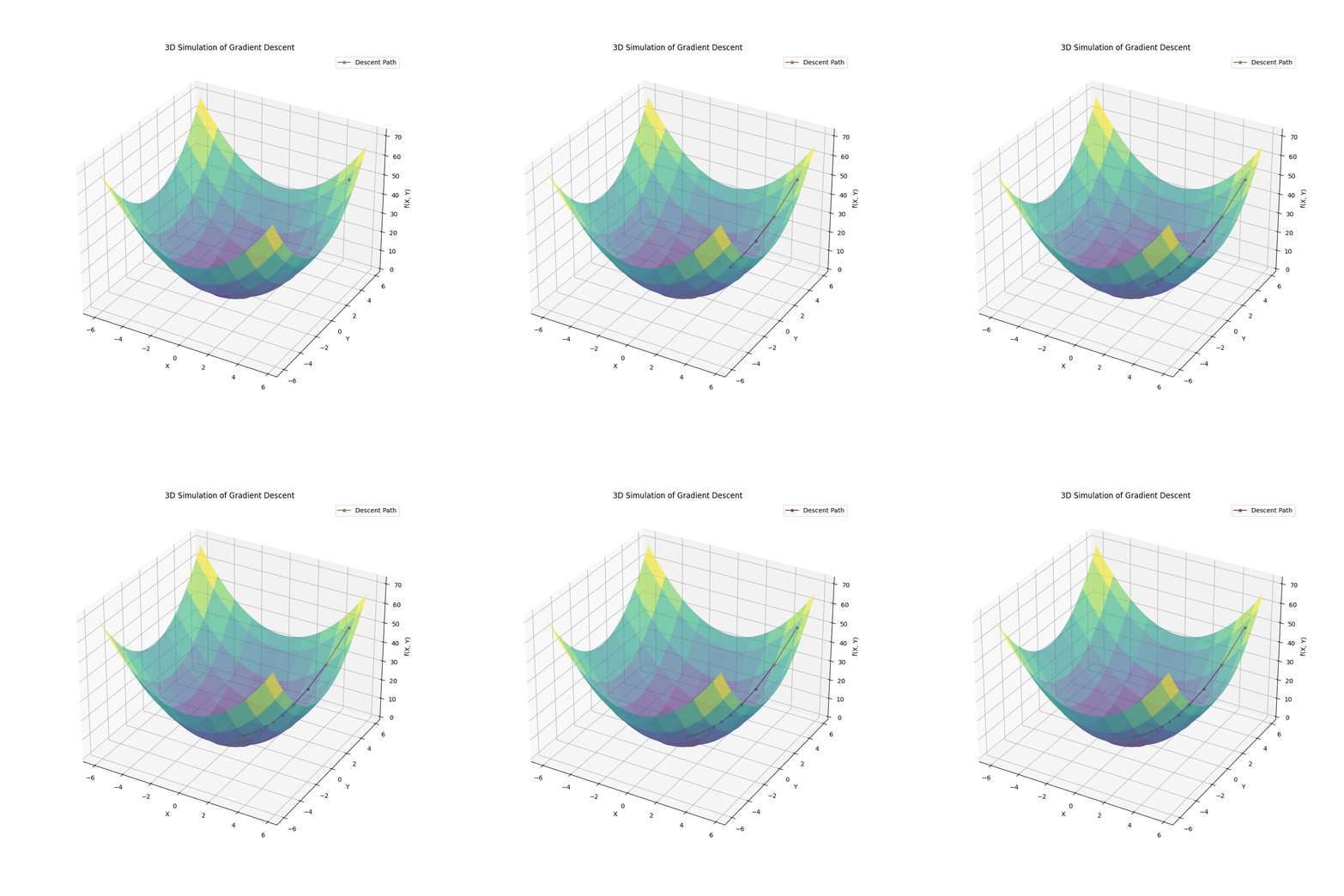
Gradient descent walking down a loss surface. Notice that the step is long where the surface is steep and short near the bottom — the gradient itself shrinks as we approach the minimum.
The learning rate: the one hyperparameter you must feel
Take the simplest possible loss, \(J(\theta) = \theta^2\), whose gradient is \(2\theta\). The update becomes
The whole behaviour of gradient descent is inside that factor \((1 - 2\eta)\). Play with the learning rate below and watch four qualitatively different worlds appear.
The transition points in that simulator are not arbitrary. For a quadratic whose curvature (second derivative) is \(L\) — the letter is for Lipschitz3 — gradient descent converges only if
Here \(L = 2\), so the boundary sits exactly at \(\eta = 1\) — try it. Below \(1/L = 0.5\) the approach is monotone; between \(1/L\) and \(2/L\) it zig-zags across the minimum; above \(2/L\) it explodes. Real loss surfaces are not quadratic, but near a minimum they look quadratic, and this bound is the reason a learning rate that worked yesterday makes today's model diverge after you changed the architecture: you changed \(L\).
Reading a training log
- Loss going down slowly and smoothly → η too small, or you are on a plateau.
- Loss going down but jittering hard → η slightly too large (or batch too small).
- Loss jumping up and down between epochs → η in the oscillating regime.
- Loss becomes
NaN→ η past the stability bound, or exploding gradients. Lower η by 10× first.
How much data per step? Batch, Stochastic and Mini-Batch
The loss over a dataset of \(N\) samples is an average of per-sample losses:
Computing \(\nabla J\) exactly means a full pass over the data for one parameter update. The three classic variants differ only in how many samples they look at before stepping.
Uses the entire dataset for every update. The gradient is exact, the trajectory is smooth — and on ImageNet you would get one update per pass over 1.2M images.
One sample per update. Each gradient is a terrible estimate of the true one, but it is unbiased4 — on average it points the right way — and you get \(N\) updates per epoch.
A small random subset of \(B\) samples — typically 32 to 512. Enough samples to make the estimate usable, few enough to keep steps cheap, and a shape the GPU can parallelize5.
The key quantitative fact: averaging \(B\) independent samples divides the standard deviation of the gradient estimate by \(\sqrt{B}\).
That square root is why batch size has diminishing returns: going from 32 to 128 costs 4× the compute per step and only halves the noise. And the noise never fully disappears — with a constant learning rate, SGD does not converge to the minimum, it converges to a cloud around the minimum whose radius grows with \(\sqrt{\eta}\) and shrinks with \(\sqrt{B}\). Watch it happen:
What the dashed circle means
It is the theoretical radius of the stationary cloud, \(r \approx \dfrac{\sigma}{\sqrt{B}}\sqrt{\dfrac{\eta}{2\mu}}\) for a quadratic with curvature \(\mu\) (one standard deviation along the flat axis). Two ways to shrink it: more data per step (bigger \(B\)) or smaller steps (smaller \(\eta\)), both only as a square root. The second one is free — which is exactly why every serious training run decays the learning rate at the end. You explore with big noisy steps early, and settle with small quiet steps late.
Batch size and learning rate move together
If you multiply the batch size by \(k\), the gradient noise drops and you can usually afford a larger step. The common heuristics are the linear scaling rule (\(\eta \to k\eta\), used to train ResNet-50 in one hour with batch 8192)6 and the square-root rule (\(\eta \to \sqrt{k}\eta\), which matches the noise argument above and tends to work better with Adam). Never change the batch size expecting the old learning rate to still be optimal.
Why plain gradient descent struggles
If the loss surface were a nice round bowl, a single learning rate would do and this chapter would end here. Real surfaces are not round, and three specific pathologies explain every optimizer that follows.
-
Ravines (ill-conditioning)
The surface is much steeper in one direction than another. The gradient points mostly across the valley instead of along it, so the iterates zig-zag between the walls while barely advancing toward the minimum.
The stability bound \(\eta < 2/L\) is set by the steepest direction, while progress along the flattest direction goes as \(\eta\mu\). The ratio \(\kappa = L/\mu\) — the condition number — is the real difficulty: convergence takes \(O(\kappa \log 1/\varepsilon)\) steps. Deep networks routinely have \(\kappa\) in the thousands.
-
Saddle points and plateaus
A point where the gradient vanishes but which is a minimum in some directions and a maximum in others. Gradient descent slows to a crawl there, because the thing driving it — the gradient — is nearly zero.
In high dimensions saddles are far more common than local minima: for a critical point to be a local minimum, all \(n\) curvature directions must be positive, and that gets exponentially unlikely as \(n\) grows. This is the modern view: the enemy is flatness, not bad minima.7
-
Noise and non-stationarity
Each mini-batch gives a slightly different gradient, and layers keep changing under each other during training, so the surface a given layer sees is not even fixed.
A good optimizer therefore has to average over time (that is momentum) and stay robust to gradients whose scale varies by orders of magnitude between layers (that is adaptivity).
One number to keep: the condition number
For \(J(x,y) = \tfrac{1}{2}(\mu x^2 + L y^2)\) with \(L \gg \mu\), the best possible learning rate is \(\eta = 2/(L+\mu)\) and the error still decays only by a factor of \(\frac{\kappa-1}{\kappa+1}\) per step. With \(\kappa = 100\) that is \(0.98\) — about 115 steps to gain a single order of magnitude, and with \(\kappa = 10\,000\) it is 11 500. Everything below is an attempt to escape that \(\kappa\).
Momentum: give the ball some weight
Instead of stepping in the direction of the current gradient, accumulate an exponential moving average of past gradients and step in that direction. Two state variables now, \(V\) and \(\theta\):
\(V\) is a running average of the gradients: at each step we dampen the old value by \(\beta\) (between 0 and 1) and mix in the new gradient. We then move \(\theta\) along the new momentum \(V\)1.
Why it fixes ravines. Across the valley the gradient flips sign every step, so consecutive terms cancel in the average and the oscillation is damped. Along the valley the sign never changes, so nothing cancels and the average settles on the gradient itself. One rule, two opposite effects on the two directions — that is the whole trick.
How much history is being averaged is set by
the effective number of past gradients in the moving average: about 10 steps at \(\beta = 0.9\), about 100 at \(\beta = 0.99\). Read it as a memory length, not a speed-up — in the form written above, once \(V\) has settled on a constant gradient the step is \(\eta V = \eta g\), exactly SGD's step. (In fact it arrives late: over a long run momentum trails plain SGD by \(\beta/(1-\beta)\) steps' worth of progress, 9 of them at \(\beta = 0.9\).)
What momentum buys, then, is not a bigger step but a better direction: what alternates cancels, what persists survives. It also keeps moving on stale gradients — which is why it coasts through small bumps, and why it can sail past a minimum instead of braking at it.
Equivalent form: the heavy ball
The next step is a combination of the previous step's direction and the new negative gradient. This is Polyak's heavy ball method8 — literally the physics of a ball with mass rolling downhill, where \(\beta\) plays the role of \(1-\text{friction}\).
Expanding the recursion turns it into \(v_{t+1} = \beta v_t + g_t\), \(\theta_{t+1} = \theta_t - \eta v_{t+1}\) — the same method as above but without the \((1-\beta)\), so its step is \(1/(1-\beta)\) times larger for the same \(\eta\). The two forms describe identical trajectories once you rescale the learning rate; which one you are holding matters enormously in practice, as the next box shows.
PyTorch does not use the formula above
torch.optim.SGD(momentum=0.9) implements
without the \((1-\beta)\) factor. The direction is identical, but the effective step is \(1/(1-\beta)\) times larger — i.e. 10× larger at \(\beta = 0.9\). This is the single most common reason a learning rate copied from a paper explodes in someone else's framework.
Nesterov: look before you leap
Nesterov Accelerated Gradient910 evaluates the gradient after the momentum step, not before:
The idea is a correction term: since we already know inertia is going to carry us to \(\theta_t - \eta\beta V_t\), we may as well measure the slope there. If the surface has started to climb again, the gradient at the look-ahead point brakes earlier than it would otherwise. In practice it gives a small but consistent improvement11, and it is one flag away: torch.optim.SGD(..., momentum=0.9, nesterov=True).
Adaptive methods: one learning rate per parameter
Momentum fixes the direction. It does not fix the fact that a single \(\eta\) has to serve every parameter in the network — the embedding of a rare word, whose gradient is almost always zero, and a bias in the first layer, whose gradient is large at every step.
The shared idea of every adaptive method: keep a per-parameter estimate of the typical gradient magnitude, and divide by it. Parameters with consistently large gradients take smaller steps; parameters with tiny gradients take larger ones. The update becomes roughly scale-free.
AdaGrad — the first idea, and its flaw
Accumulate the sum of all squared gradients seen so far and divide by its square root12:
This works beautifully for sparse features and it is where the whole family starts. But \(G_t\) is a sum that never decreases, so the effective learning rate \(\eta/\sqrt{G_t}\) decays monotonically toward zero. On a long deep-learning run, AdaGrad stops learning long before it has converged.
RMSProp — replace the sum by a moving average
The fix13 is one character wide: turn the sum into an exponential moving average, so old gradients are forgotten.
where:
- \(V_t\) is the moving average of the squared gradients (typically \(\beta = 0.9\); PyTorch calls it
alphaand defaults to0.99), - \(\epsilon \approx 10^{-8}\) is a small constant for numerical stability, preventing division by zero.
Now \(\sqrt{V_t}\) is the root mean square of the recent gradients — hence the name — and it tracks the current terrain instead of the whole history. Note that \(g/\sqrt{\overline{g^2}}\) is dimensionless and roughly \(\pm 1\): RMSProp is close to "take a step of size \(\eta\) in the sign of the gradient", which is precisely what makes it immune to a badly scaled loss.
Adam — momentum and RMSProp in one
Adaptive Moment Estimation keeps both moving averages: the first moment (the mean of the gradients — momentum) and the second moment (the uncentered variance — RMSProp).
-
Compute the gradient:
\[g_t = \nabla J(\theta_t)\] -
First moment (direction, with inertia):
\[m_t = \beta_1 m_{t-1} + (1 - \beta_1) g_t\] -
Second moment (scale):
\[v_t = \beta_2 v_{t-1} + (1 - \beta_2) g_t^2\] -
Bias correction:
\[\hat{m}_t = \frac{m_t}{1 - \beta_1^t}, \qquad \hat{v}_t = \frac{v_t}{1 - \beta_2^t}\] -
Update:
\[\theta_{t+1} = \theta_t - \eta \, \frac{\hat{m}_t}{\sqrt{\hat{v}_t} + \epsilon}\]
where \(\beta_1, \beta_2\) control the decay of the two averages and \(\epsilon\) guards the division. The defaults are \(\beta_1 = 0.9\), \(\beta_2 = 0.999\), \(\epsilon = 10^{-8}\)1415, and they are remarkably robust — Adam is the closest thing we have to an optimizer that works out of the box.
Why the bias correction? A worked example
Both averages start at zero, so early on they are biased toward zero — and, crucially, by different amounts, because \(\beta_1 \ne \beta_2\).
Suppose the gradient is a constant \(g = 1\). At the very first step:
| value at \(t=1\) | corrected | |
|---|---|---|
| \(m_1 = (1-\beta_1)g\) | \(0.1\) | \(\hat{m}_1 = 0.1/(1-0.9) = 1.0\) |
| \(v_1 = (1-\beta_2)g^2\) | \(0.001\) | \(\hat{v}_1 = 0.001/(1-0.999) = 1.0\) |
Without correction the step would be \(\eta \cdot \dfrac{0.1}{\sqrt{0.001}} = 3.16\,\eta\) — more than three times too large, right at the start of training, when the model is most fragile. With correction it is exactly \(\eta \cdot \dfrac{1.0}{\sqrt{1.0}} = \eta\), the step you asked for.
Both factors go to 1 as \(t\) grows, but at very different rates: \(1-\beta_1^t\) is within 1% of 1 by step 44, while \(1-\beta_2^t\) needs about 4 600 steps (\(0.999^{1000} \approx 0.37\), so the second-moment correction is still doing real work well into training). The correction matters most at the start — which is why it and warmup (next section) address overlapping problems.
Adam is the default for training deep networks: it combines momentum's smoothing with per-parameter adaptivity, and it needs far less learning-rate tuning than SGD. The price is memory — two extra tensors the size of the model — and a well-documented tendency to generalize slightly worse than well-tuned SGD+momentum on convolutional vision tasks.16
AdamW — decoupled weight decay
AdamW17 separates weight decay from the adaptive update, which is mathematically the correct thing to do:
where \(\lambda\) is the weight-decay coefficient applied directly to the weights, not to the gradient.
In the original Adam, L2 regularization is implemented by adding \(\lambda\theta\) to the gradient before the adaptive scaling — so it gets divided by \(\sqrt{\hat{v}_t}\) too. The consequence is perverse: parameters with large gradients end up being regularized less, which is the opposite of what you want. AdamW applies the decay outside the adaptive term, restoring the intended behaviour. It is the standard for training Transformers and LLMs (BERT, GPT, LLaMA), usually with \(\lambda \approx 0.01\)–\(0.1\).
Do not decay every parameter
Weight decay is meant for weight matrices. Biases, and the gain/bias of LayerNorm and BatchNorm, should be excluded — decaying them hurts with no regularization benefit. Every serious training script splits the parameters into two groups for exactly this reason.
Simulator: the optimizer race
Everything above, side by side. Pick a landscape, set the learning rate, and watch five optimizers start from the same point. The bottom panel shows the loss on a logarithmic scale — the shape of those curves is what you actually see in a training log.
What to look for
Some experiments worth running:
- Ravine, η just above the default. SGD is the first to explode: its stability limit is \(2/L = 0.4\), dictated by the steep direction alone. The adaptive methods keep going well past it, because dividing by \(\sqrt{v_t}\) scales that direction back down. Note also that RMSProp never quite settles — with no momentum, its step stays around \(\eta\) and it hovers around the minimum instead of landing on it.
- Saddle, default η. SGD and Momentum are still sitting on the ridge after 300 steps — the escape gradient there is ~0.004, and a step proportional to the gradient is essentially no step at all. RMSProp and Adam divide by the gradient's own magnitude, so their step stays close to \(\eta\) and they reach the minimum in a few dozen steps. This is the practical reason adaptive methods deal so well with plateaus.
- Non-convex, η at 1×, then 2× and 4×. At the default everyone is trapped in the nearest dip — the basin was decided in the first few steps, which is why initialization matters. Push η up and the normalized methods (Adam first, then RMSProp) take steps wide enough to clear a ridge (at 4× Momentum's inertia clears one too), while SGD stays exactly where it landed. Note what this implies: what escapes a bad region is a big enough step, not intelligence — and in real training that role is played by the mini-batch noise from the previous simulator.
- AdaGrad on the saddle or on Rosenbrock, long run. Watch it slow down and stop — the purple curve flattens out while RMSProp keeps going. That is the accumulated \(G_t\) strangling the step size.
- Rosenbrock at 4× η. SGD diverges while Momentum and Adam ride the curved valley to \((1,1)\). At the default η nobody arrives within 300 steps, and AdaGrad never arrives at all — the honest picture of a badly conditioned problem, and the reason second-order methods still exist.
A caveat about racing optimizers
These are 2-parameter deterministic problems. Real networks have millions of parameters, noisy gradients and a surface that changes as the layers co-adapt. Use these pictures for intuition about mechanisms — oscillation, inertia, rescaling — not as evidence that one optimizer beats another. On real tasks, a well-tuned SGD+momentum still wins some benchmarks that Adam loses.
Learning rate schedules
The noise simulator showed why a constant learning rate cannot be optimal: big steps explore fast but leave you orbiting the minimum; small steps settle precisely but take forever to get there. So do both — start big, end small.
Two extra ingredients matter in practice. Warmup ramps \(\eta\) up from ~0 over the first few hundred/thousand steps: at initialization the gradients are large and Adam's second moment estimate is still garbage, so full-size steps early can wreck the model — this is essential for Transformers18. And cosine decay brings \(\eta\) smoothly to zero by the end of training, which empirically beats step decay on almost everything.19
import torch, math

opt = torch.optim.AdamW(model.parameters(), lr=3e-4, weight_decay=0.01)

warmup, total = 500, 10_000
def factor(step):                                   # returns a multiplier on lr
    if step < warmup:
        return (step + 1) / warmup                  # linear ramp up (never exactly 0)
    p = (step - warmup) / (total - warmup)          # progress in [0, 1]
    return 0.5 * (1 + math.cos(math.pi * p))        # cosine down to 0

sched = torch.optim.lr_scheduler.LambdaLR(opt, factor)

for x, y in loader:
    loss = criterion(model(x), y)
    opt.zero_grad(set_to_none=True)
    loss.backward()
    torch.nn.utils.clip_grad_norm_(model.parameters(), 1.0)   # see below
    opt.step()
    sched.step()                                    # per step, not per epoch
Gradient clipping
One bad mini-batch can produce a gradient hundreds of times larger than usual — and one such step can undo an hour of training. Clipping rescales the whole gradient whenever its norm exceeds a threshold:
The direction is preserved, only the length is capped. With \(c = 1.0\) it costs nothing and it is standard practice for RNNs, Transformers and any model trained in mixed precision.20
Choosing an optimizer in practice
Side by side
| Batch GD | SGD / Mini-batch | Momentum | RMSProp | Adam / AdamW | |
|---|---|---|---|---|---|
| Direction | exact gradient | noisy gradient | moving average of gradients | gradient, rescaled | averaged gradient, rescaled |
| Step size | fixed η | fixed η | fixed η (×\(\frac{1}{1-\beta}\) in PyTorch's convention) | per parameter | per parameter |
| Cost per update | high (full dataset) | low (one mini-batch) | low (same as SGD, + 1 buffer) | low (+ 1 buffer) | medium (+ 2 buffers) |
| Extra memory | — | — | 1× model | 1× model | 2× model |
| Handles ravines | poorly | poorly | well | well | very well |
| Escapes saddles | no | by noise | by inertia | well | well |
| Sensitivity to η | high | high | high | medium | low |
| Typical use | small convex problems | vision with a good schedule | CNNs, RL | RNNs, non-stationary losses | Transformers, LLMs, default |
| Hyperparameters | η | η, batch size | η, β ≈ 0.9 | η ≈ 1e-3, β ≈ 0.9 | η ≈ 1e-3, β₁ = 0.9, β₂ = 0.999, λ |
| Main weakness | one update per epoch | oscillation, needs tuning | can overshoot | no momentum | memory; sometimes generalizes worse than SGD |
In short: Batch GD is exact but impractical; SGD buys speed with noise; Momentum smooths that noise and accelerates along consistent directions; RMSProp fixes the scale of each parameter; and Adam/AdamW combines the last two, which is why it is the default — although a well-tuned SGD+momentum still generalizes better on some vision benchmarks.
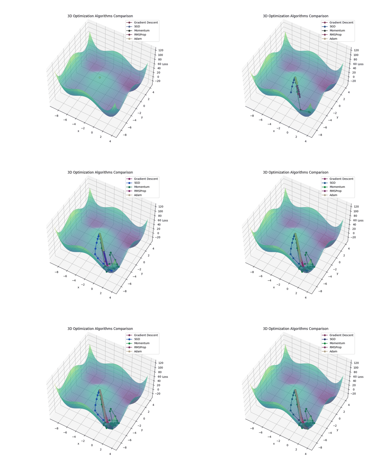
The same start, five optimizers, 50 steps. All of them slide off the flat hilltop where they start and settle in the same minimum: RMSProp turns first, Momentum overshoots and swings back, and Adam, whose step stays near η, arrives last.
The right choice depends on the size of the dataset, the compute available and how much tuning you can afford — validate on held-out data rather than trusting a table.
Sensible defaults
| Situation | Optimizer | Starting point |
|---|---|---|
| Transformer / LLM, from scratch | AdamW | lr=3e-4, betas=(0.9, 0.95), wd=0.1, warmup + cosine |
| Fine-tuning a pretrained model | AdamW | lr=2e-5 to 5e-5, wd=0.01, short warmup |
| CNN on images, long training | SGD + Nesterov | lr=0.1 (batch 256), momentum=0.9, wd=5e-4, cosine |
| MLP on tabular data | Adam | lr=1e-3, defaults for everything else |
| Anything, first attempt | Adam | lr=1e-3 — then tune the learning rate before anything else |
The only hyperparameter search that always pays off
Sweep the learning rate over powers of ten (1e-1, 1e-2, 1e-3, 1e-4), train for a few hundred steps each, and keep the largest one that does not blow up — then halve it. Tuning \(\beta_1\), \(\beta_2\) or \(\epsilon\) before doing this is wasted effort: their defaults are good, and \(\eta\) dominates everything.
Troubleshooting a training run
| Symptom | Likely cause | What to try |
|---|---|---|
Loss is NaN / inf | η above the stability bound, exploding gradients, log(0) in the loss | ÷10 on η, add gradient clipping, check the loss for numerical issues |
| Loss flat from step 0 | η far too small, dead ReLUs, broken data pipeline | ×10 on η; verify the model can overfit 10 samples |
| Loss drops then plateaus high | stuck on a plateau / saddle, or η now too large for this phase | add momentum, decay η, check initialization |
| Train loss fine, val loss rising | overfitting — not an optimizer problem | weight decay, dropout, augmentation, early stopping |
| Loss jitters violently | batch too small or η too large | increase batch size, decay η, add momentum |
| Fine at first, diverges at epoch k | learning rate too high for the sharper region reached later | schedule the learning rate; add warmup |
The optimizers, from scratch
All of them are ten lines. Written side by side, the family resemblance is obvious — every one is θ -= η · (direction) / (scale).
import numpy as np

class SGD:
    def __init__(self, lr=0.01, beta=0.0):
        self.lr, self.beta, self.v = lr, beta, None

    def step(self, theta, grad):
        if self.v is None:
            self.v = np.zeros_like(theta)
        self.v = self.beta * self.v + (1 - self.beta) * grad     # momentum (beta=0 → plain SGD)
        return theta - self.lr * self.v


class RMSProp:
    def __init__(self, lr=0.01, beta=0.9, eps=1e-8):
        self.lr, self.beta, self.eps, self.v = lr, beta, eps, None

    def step(self, theta, grad):
        if self.v is None:
            self.v = np.zeros_like(theta)
        self.v = self.beta * self.v + (1 - self.beta) * grad ** 2   # average squared magnitude
        return theta - self.lr * grad / (np.sqrt(self.v) + self.eps)


class Adam:
    def __init__(self, lr=1e-3, b1=0.9, b2=0.999, eps=1e-8, weight_decay=0.0):
        self.lr, self.b1, self.b2, self.eps, self.wd = lr, b1, b2, eps, weight_decay
        self.m = self.v = None
        self.t = 0

    def step(self, theta, grad):
        if self.m is None:
            self.m = np.zeros_like(theta)
            self.v = np.zeros_like(theta)
        self.t += 1
        self.m = self.b1 * self.m + (1 - self.b1) * grad            # 1st moment: direction
        self.v = self.b2 * self.v + (1 - self.b2) * grad ** 2       # 2nd moment: scale
        m_hat = self.m / (1 - self.b1 ** self.t)                    # bias correction
        v_hat = self.v / (1 - self.b2 ** self.t)
        update = m_hat / (np.sqrt(v_hat) + self.eps)
        return theta - self.lr * (update + self.wd * theta)         # AdamW: decay outside the scaling
# The same thing, in PyTorch
torch.optim.SGD(p, lr=0.1, momentum=0.9, nesterov=True, weight_decay=5e-4)
torch.optim.RMSprop(p, lr=1e-3, alpha=0.9)
torch.optim.Adam(p, lr=1e-3, betas=(0.9, 0.999), eps=1e-8)
torch.optim.AdamW(p, lr=3e-4, betas=(0.9, 0.95), weight_decay=0.1)
Key takeaways
- Gradient descent is one line; everything else is about choosing the step size well.
- A quadratic converges only when \(\eta < 2/L\). Divergence is not bad luck, it is arithmetic.
- Mini-batches trade noise for speed, and the noise falls only as \(1/\sqrt{B}\). A constant learning rate leaves you orbiting the minimum — hence schedules.
- The real obstacles are ill-conditioning and saddle points, not bad local minima.
- Momentum averages gradients over time, so what alternates cancels and what persists survives. \(1/(1-\beta)\) is the length of that memory — and, in PyTorch's convention, also the factor by which the step grows.
- Adaptive methods (AdaGrad → RMSProp → Adam) give every parameter its own step size by dividing by the RMS of recent gradients. Adam adds momentum and bias correction on top.
- AdamW + warmup + cosine is the modern default. Tune the learning rate first, and almost nothing else.
Additional Resources
Three things that carry on from where this page stops, in the order that makes sense:
-
Who's Adam and What's He Optimizing? — Kundu, S. Walks the same road as this chapter — SGD, momentum, RMSProp, Adam — in animation. The fastest way to revise the whole page:
-
An overview of gradient descent optimization algorithms — Ruder, S. Gathers every method here into one notation, plus the ones left out (Adadelta, Nadam, AMSGrad). Read it once the chapter is closed, to see the full map.
-
Why Momentum Really Works — Goh, G., Distill (2017). An entirely interactive article on what the condition number does to convergence. The natural next step after the momentum section: it proves with sliders what is left as intuition here.
References
The works cited through the text, in order of appearance:
-
Introduction to Gradient Descent and Backpropagation Algorithm — LeCun, Y., NYU Deep Learning course notes. ↩↩↩
-
Formally, the rate at which \(J\) changes as you move in a unit direction \(u\) is the directional derivative \(D_u J = \nabla J \cdot u = \lVert \nabla J \rVert \cos\alpha\), where \(\alpha\) is the angle between \(u\) and \(\nabla J\). Only the cosine depends on \(u\), so the value is largest at \(\alpha = 0\) (with \(u\) aligned to \(\nabla J\)) and smallest at \(\alpha = 180°\) (with \(u = -\nabla J / \lVert \nabla J \rVert\)). That is the argument guaranteeing the gradient is the direction of steepest ascent, not merely an ascending direction. ↩
-
Lipschitz is Rudolf Lipschitz (1832–1903), a German mathematician. A function is Lipschitz continuous with constant \(L\) when it never changes faster than \(L\): take any two points \(x\) and \(y\), and \(\lvert f(x) - f(y) \rvert \le L \lvert x - y \rvert\). In words, the straight line joining any two points of the graph has slope at most \(L\) in absolute value — the function has a speed limit, and \(L\) is that limit. What is Lipschitz here is not the loss but its gradient: \(\lVert \nabla J(x) - \nabla J(y) \rVert \le L \lVert x - y \rVert\), which says the slope itself cannot change faster than \(L\), and a bound on how fast the slope changes is exactly a bound on the curvature (\(L\) is the largest eigenvalue of the Hessian in absolute value, when \(J\) is twice differentiable). That is the intuition behind \(\eta < 2/L\): the gradient you measured at \(\theta_t\) only describes the surface well for a while, and the faster it is allowed to change, the shorter the step you may take. ↩
-
Robbins, H., & Monro, S. (1951). A Stochastic Approximation Method — Annals of Mathematical Statistics 22(3), 400–407. The origin of stochastic approximation: the proof that noisy estimates of the gradient are enough, provided the step sizes shrink at the right rate. ↩
-
Stochastic and Mini-batch Gradient Descent — Watt, J., Borhani, R., & Katsaggelos, A., Machine Learning Refined. ↩
-
Goyal, P., Dollár, P., Girshick, R., et al. (2017). Accurate, Large Minibatch SGD: Training ImageNet in 1 Hour — where the linear scaling rule and gradual warmup were established, at batch 8192. ↩
-
Dauphin, Y., Pascanu, R., Gulcehre, C., et al. (2014). Identifying and Attacking the Saddle Point Problem in High-Dimensional Non-Convex Optimization — NeurIPS. The paper behind the claim that saddles, not local minima, dominate in high dimension. ↩
-
Polyak, B. T. (1964). Some methods of speeding up the convergence of iteration methods — USSR Computational Mathematics and Mathematical Physics 4(5), 1–17. The heavy ball, 22 years before backpropagation. ↩
-
Nesterov, Y. (1983). A method for solving the convex programming problem with convergence rate \(O(1/k^2)\) — Doklady Akademii Nauk SSSR 269, 543–547. The original acceleration result; it predates its use in neural networks by three decades. ↩
-
Optimization, the Philosophical Background of Artificial Intelligence — Nesterov, Y., talk at ICBS 2024. Not about the method itself: it is him on where optimization sits inside AI. ↩
-
Sutskever, I., Martens, J., Dahl, G., & Hinton, G. (2013). On the importance of initialization and momentum in deep learning — ICML. The paper that brought Nesterov's acceleration into deep learning practice, and measured how much it and the initialization matter. ↩
-
Duchi, J., Hazan, E., & Singer, Y. (2011). Adaptive Subgradient Methods for Online Learning and Stochastic Optimization — JMLR 12, 2121–2159. AdaGrad, and the per-parameter learning rate the rest of the family inherits. ↩
-
Tieleman, T., & Hinton, G. (2012). Lecture 6.5 — RMSProp: divide the gradient by a running average of its recent magnitude — Coursera, Neural Networks for Machine Learning. RMSProp has no paper: these slides are what everyone cites. ↩
-
Kingma, D. P., & Ba, J. (2015). Adam: A Method for Stochastic Optimization — ICLR. ↩
-
Dive into Deep Learning — Zhang, A., Lipton, Z. C., Li, M., & Smola, A. J. Chapter 12 derives every optimizer on this page, with code. ↩
-
Wilson, A. C., Roelofs, R., Stern, M., Srebro, N., & Recht, B. (2017). The Marginal Value of Adaptive Gradient Methods in Machine Learning — NeurIPS. The systematic evidence for the generalization gap between Adam and tuned SGD. ↩
-
Loshchilov, I., & Hutter, F. (2019). Decoupled Weight Decay Regularization — ICLR. AdamW. ↩
-
Vaswani, A., Shazeer, N., Parmar, N., et al. (2017). Attention Is All You Need — NeurIPS. Section 5.3 defines the warmup-then-\(1/\sqrt{t}\) schedule the simulator plots as "Noam". ↩
-
Loshchilov, I., & Hutter, F. (2017). SGDR: Stochastic Gradient Descent with Warm Restarts — ICLR. Where cosine annealing comes from. ↩
-
Pascanu, R., Mikolov, T., & Bengio, Y. (2013). On the difficulty of training recurrent neural networks — ICML. Where norm clipping comes from, and why exploding gradients happen at all. ↩