7. Regularization

A model that fits the training data perfectly is not the goal — it is a warning sign. What we actually want is a model that does well on data it has never seen, and those two things pull in opposite directions. Regularization is the name for every technique that deliberately makes the training fit worse in exchange for a better fit on everything else.

Formally, training minimizes the loss we can measure, over the \(N\) examples we happen to have:

\[ \hat{R}(\theta) = \frac{1}{N}\sum_{i=1}^{N} L\big(f_\theta(x^{(i)}), y^{(i)}\big) \]

but what we care about is the loss over the whole distribution the data came from, which we cannot measure:

\[ R(\theta) = \mathbb{E}_{(x,y)\sim \mathcal{D}}\big[L(f_\theta(x), y)\big] \]

The difference \(R(\theta) - \hat{R}(\theta)\) is the generalization gap, and every technique in this chapter is an attempt to keep it small.

Seeing it happen

Nothing explains overfitting like watching it. Below, 12 noisy points are drawn from a smooth function, and a polynomial of the degree you choose is fitted to them by least squares. The dashed line is the truth we are trying to recover; the crosses are held-out points the fit never saw.

degree 1 L2 penalty λ 0 training points 12

Three experiments worth running, in order:

Degree 1, then 3, then 14, with \(\lambda = 0\). Degree 1 cannot bend at all. Degree 3 lands close to the truth. Degree 14 threads every single training point — train error collapses to essentially zero — and lurches violently between them. That is overfitting: not a model that is wrong, but a model that is right about the noise.
Stay at degree 14 and raise \(\lambda\). Nothing about the model shrinks; it still has 15 coefficients. But the wild curve calms down and the held-out error drops. Capacity was never the problem — unconstrained capacity was.
Stay at degree 14, \(\lambda = 0\), and drag the number of points up. The same model that was useless with 12 points becomes reasonable with 60. More data is regularization too, and the most effective kind.

Watch ‖w‖² in the readout

Sweep the degree at 12 points and follow the coefficients: \(\lVert w \rVert^2\) goes from about \(5\) at degree 3 to \(5\times10^{5}\) at degree 14. Enormous coefficients of alternating sign are exactly how a curve produces those violent swings between points, and that observation is what every penalty method in this chapter is built on: at a fixed amount of data, huge weights are the signature of a model that is memorizing.

The qualifier matters. Raise the data to 60 points and degree 14 generalizes well while still having a huge norm — so the norm is not a verdict on its own, which is why bounds based only on weight size explain much less about deep networks than we would like¹.

Bias and variance

The two failures in that simulator have names, and they come from splitting the expected error of a model into pieces. For squared loss, at a point \(x\), averaging over all training sets we might have drawn:

\[ \mathbb{E}\big[(y - \hat{f}(x))^2\big] \;=\; \underbrace{\big(\mathbb{E}[\hat{f}(x)] - f(x)\big)^2}_{\text{bias}^2} \;+\; \underbrace{\mathbb{E}\big[(\hat{f}(x) - \mathbb{E}[\hat{f}(x)])^2\big]}_{\text{variance}} \;+\; \underbrace{\sigma^2}_{\text{noise}} \]

Read the three terms as three different complaints:

Bias — the model is systematically wrong, in the same way, no matter which training set it gets. The degree-1 fit is biased: it cannot bend, so it misses the curve every time.
Variance — the model changes wildly depending on which training set it happened to see. The degree-14 fit has enormous variance: resample the 12 points and you get a completely different curve.
Noise — the irreducible part, \(\sigma^2 = 0.032\) in the simulator. No model beats it, and a model that scores below it on training data is fitting noise by definition.

Model capacity trades the first against the second, which is the classic bias-variance tradeoff:

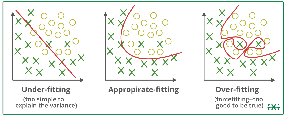
Underfitting and overfitting. Source: GeeksforGeeks²

Too much bias (underfitting)

Train and validation error are both high and close to each other.
- Increase capacity: more layers, more units.
- Train longer — you may simply not have converged.
- Add or engineer features; check the data pipeline.
- Reduce the regularization you already have.
Too much variance (overfitting)

Train error is low, validation error is much higher. The gap is the symptom.
- More data, or augmentation to simulate more data.
- Penalize the weights (L1/L2), add dropout, stop early.
- Reduce capacity — the last resort, not the first.
- Check for leakage before believing any of this.

The U-curve is not the whole story any more

The classic picture says test error falls, bottoms out, then rises forever as capacity grows. Modern networks break it: push capacity past the point where the model interpolates the training set perfectly and test error often falls again, sometimes below the first minimum. This is double descent³⁴, and it is why "just make the model smaller" is bad advice for deep networks. The curve you were taught still describes the underparameterized regime — most deep networks simply do not live there.

Penalizing the weights: L1 and L2

The simulator's lesson was that memorizing needs enormous coefficients. So add their size to the loss and let the optimizer weigh the two objectives:

L2 (ridge, weight decay)L1 (lasso)

\[ \tilde{J}(w) = J(w) + \frac{\lambda}{2}\sum_i w_i^2 \]

The gradient of the penalty is \(\lambda w\), so a gradient step becomes

\[ w \leftarrow w - \eta\nabla J(w) - \eta\lambda w = \underbrace{(1 - \eta\lambda)}_{\text{shrink}} w - \eta \nabla J(w) \]

Every step multiplies the weights by a factor slightly below 1 before the gradient is applied — which is exactly why the same idea is called weight decay⁵. Weights survive only if the gradient keeps pushing them back up, so the penalty acts as constant pressure toward zero that useful weights must earn their way out of.

\[ \tilde{J}(w) = J(w) + \lambda\sum_i |w_i| \]

The gradient of the penalty is \(\lambda\,\mathrm{sign}(w)\) — the same size no matter how small \(w\) is. Where L2 pushes proportionally (and so pushes ever more gently as the weight shrinks), L1 pushes with constant force all the way to zero, and holds it there.

The result is exact zeros, not just small values: L1 performs feature selection as a side effect of the optimization⁶.

Why L1 gives you zeros and L2 does not

This is easier to see than to prove. Below, the ellipses are the contours of the unregularized loss and the shaded region is what the penalty allows; the penalized solution sits where the smallest ellipse touches that region. Drag the black dot — the unregularized optimum — and watch what each penalty does with it.

penalty strength λ 0.30 drag the black dot to move the unregularized optimum

The shapes are the whole argument. The L2 region is a circle, which is smooth everywhere, so the point where it first touches an ellipse is almost never on an axis — both coordinates end up small but alive. The L1 region is a diamond, and a diamond is all corners; the corners lie on the axes, and a shrinking ellipse hits a corner for a wide range of directions it could have come from. That is sparsity: not a numerical accident, but a consequence of the shape.

Try dragging \(\hat{w}\) close to one axis and raising \(\lambda\) — the L1 solution snaps onto the axis and stays there, while the L2 solution slides toward the origin without ever arriving.

Weight decay is not L2 penalty once you use Adam

Adding \(\frac{\lambda}{2}\lVert w \rVert^2\) to the loss and decaying the weights by \((1-\eta\lambda)\) each step are the same operation for plain SGD — as the derivation above shows. They stop being the same the moment the optimizer rescales the gradient per parameter, because the penalty gets rescaled along with it. That is precisely the bug AdamW fixes, and it is covered in the optimization chapter. In PyTorch: torch.optim.AdamW(..., weight_decay=0.01) decays; Adam(..., weight_decay=0.01) penalizes, and they do not mean the same thing.

Do not penalize everything

Penalize weight matrices. Leave out the biases (they shift, they do not scale, and shrinking them just biases the output) and the gain/offset of every normalization layer (shrinking \(\gamma\) toward 0 fights the very thing the layer is there to do). Typical \(\lambda\): \(10^{-5}\) to \(10^{-2}\) for SGD-trained CNNs, \(0.01\)–\(0.1\) for AdamW-trained Transformers.

Dropout: break the co-adaptations

Dropout⁷ attacks a different failure. A network can memorize by building co-adapted groups of neurons: detectors that only work because some other specific neuron is there to correct them. Such a committee is brittle, and it is exactly what fails on new data.

The fix is brutal. At every training step, each unit is deleted independently with probability \(p\):

\[ m_j \sim \text{Bernoulli}(1-p), \qquad \tilde{h}_j = \frac{m_j}{1-p}\, h_j \]

No unit can rely on any other being present, because any of them may be gone on the next step. Each neuron is forced to be useful on its own, and the network stops putting all its confidence in a few fragile paths.

There is a second reading of the same equation. Every mask is a different thinned subnetwork, and with \(n\) units there are \(2^n\) of them sharing weights. Training with dropout trains that whole ensemble a little at a time, and testing without it approximates averaging their predictions — an ensemble at the price of a single model.

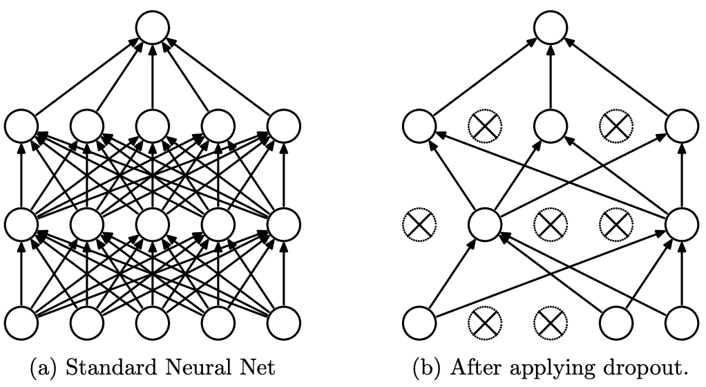
Left: a standard net with two hidden layers. Right: one thinned net produced by dropout; the crossed units were dropped for that step. Source: Srivastava et al.⁷

The \(1/(1-p)\) everyone gets wrong

Deleting units at training time lowers the expected value of what the next layer receives. That has to be compensated, and there are two ways to do it:

	when	what happens at test time
Original dropout (2014 paper)	multiply weights by \(1-p\) at test time	inference must know \(p\) and rescale
Inverted dropout (what everyone implements)	divide by \(1-p\) during training	nothing — inference is a plain forward pass

Every framework in use today does the inverted version, which is why model.eval() simply turns dropout off rather than rescaling anything. Watch the expectation being preserved:

drop probability p 0.50

Let it run: the average of the training output converges to the inference output, whatever \(p\) is. That is the entire point of dividing by \(1-p\) — the next layer sees the same expected input in both modes, so the network you train is the network you deploy. Push \(p\) to 0.9 and watch the average take much longer to settle: heavy dropout preserves the mean but adds enormous variance, which is why it slows convergence.

Forgetting model.eval()

Dropout active at inference makes predictions random, and batch normalization keeps updating its running statistics. It is the most common bug in student code — and it does not crash, it just quietly makes results worse and irreproducible. Always model.eval() for validation and inference, model.train() to go back.

Where dropout is used today


Fully connected layers	Its home ground. \(p = 0.2\)–\(0.5\)
Convolutional layers	Rarely, and with small \(p\); the weight sharing already regularizes, and BatchNorm competes
Transformers	Yes, but modestly (\(p = 0.1\) typical) on attention and MLP blocks, plus stochastic depth
Output layer	Never
Input layer	Occasionally, with small \(p\) (10–20%) — closer to data augmentation than to dropout

Dropout and BatchNorm disagree

Placed together, they fight: dropout changes the variance of the activations between training and inference, while BatchNorm memorized statistics from the training regime. The mismatch is documented⁸, and the practical rules that came out of it are to put dropout after the normalization layer, never between convolution and BN, and to use less of both than you would use of either alone. When modern architectures pick one, they usually pick normalization.

Normalization layers

Batch normalization⁹ standardizes the input of a layer using the statistics of the current mini-batch:

\[ \hat{x} = \frac{x - \mu_B}{\sqrt{\sigma_B^2 + \epsilon}}, \qquad y = \gamma \hat{x} + \beta \]

where \(\mu_B\) and \(\sigma_B^2\) are the mean and variance over the batch, and \(\epsilon \approx 10^{-5}\) keeps the root away from zero. The learned \(\gamma\) and \(\beta\) then let the layer undo the normalization if that is what helps — including recovering the identity, so the layer can never cost the network representational power.

The \(\epsilon\) goes inside the square root

\(\dfrac{x-\mu}{\sqrt{\sigma^2+\epsilon}}\), not \(\dfrac{x-\mu}{\sigma+\epsilon}\). The second form is a common typo and it is not equivalent: it changes the scale of every activation by a quantity that depends on \(\sigma\), instead of merely guarding a division.

Training and inference are different computations

This is the part that trips people up, and it is worth being exact about, because it is also where the regularizing effect comes from.

	statistics used	\(\gamma,\beta\)	running stats
Training (`model.train()`)	mean/variance of the current batch	learned	updated
Inference (`model.eval()`)	fixed running averages collected during training	learned	frozen

At training time a sample's normalized value depends on which other samples landed in its batch — so the same image gets a slightly different representation depending on its company. That is noise injected into the forward pass, and it is why batch normalization regularizes at all. At inference the batch is gone and the network must be deterministic, so the stored averages take over.

Note what this does not say: batch normalization is not "turned off" at inference. It always runs — it just switches which statistics it uses. Turning it off would change the scale of every activation and destroy the model.

Why it works — not the reason originally given

The original paper explained the benefit as reducing internal covariate shift: the drift in each layer's input distribution as the layers below it learn. That story was tested directly and did not hold — a network with noise deliberately injected after normalization, so the shift is restored, trains just as well¹⁰. The current explanation is that normalization makes the loss surface smoother and its gradients more predictable, which is what allows the larger learning rates. The technique works; the mechanism in the 2015 abstract does not.

LayerNorm, and why Transformers use it instead

Batch normalization has a structural weakness: it needs a batch. That breaks with batch size 1, with variable-length sequences, and it makes training and inference behave differently by construction.

LayerNorm¹¹ normalizes over the features of a single sample instead of over the batch:

\[ \mu = \frac{1}{d}\sum_{j=1}^{d} x_j, \qquad \sigma^2 = \frac{1}{d}\sum_{j=1}^{d}(x_j - \mu)^2 \]

Each sample is now normalized by its own statistics. There is nothing to average across the batch, so there are no running statistics, training and inference are the same computation, and batch size is irrelevant. That is why every Transformer uses it — and also why LayerNorm does not regularize: no batch, no noise from the batch composition.

Stopping early

Train long enough on a model with spare capacity and it will begin to fit the noise. Validation loss records the moment: it falls with the training loss for a while, bottoms out, and then rises while the training loss keeps going down. Early stopping is the decision to keep the model from the bottom of that curve.

The recipe has three parts, and the third is the one people forget:

Evaluate on a validation split every epoch (or every \(k\) steps).
Patience¹² — how many evaluations without improvement you tolerate before stopping. Too small and you quit on noise; too large and you waste compute past the point of no return.
Restore the best checkpoint. Stopping is not enough — the weights in memory when you stop are the worse ones, from patience epochs past the minimum. Keep a copy of the best.

Below, a degree-15 polynomial is fitted to 10 noisy points by plain gradient descent. Nothing is penalized and nothing is dropped; the only thing that varies is when you stop.

patience (epochs without improvement) 200

The right-hand panel is the point: one training run, two very different models. The green curve — the one you keep — follows the truth. The red one cost ninety times more compute (20 000 epochs against 225), threads every training point, and is worse everywhere in between. Its training loss is genuinely lower. That is the whole trap.

Early stopping is regularization, in a precise sense

It is not a heuristic bolted on the side. For a linear model trained by gradient descent from zero, stopping after \(t\) steps yields almost exactly the ridge solution with \(\lambda \approx 1/(\eta t)\): gradient descent picks up the well-determined directions of the data first and the noisy, poorly-determined ones last, so stopping early leaves the latter near zero — the same thing the L2 penalty does explicitly¹³. Training longer and regularizing less are two names for one dial.

More data, and how to manufacture it

Go back to the first simulator and drag the number of points from 12 to 60 with degree 14 and no penalty. The model that was useless becomes fine. Nothing about the model changed — the constraint came from the data. This is worth stating plainly, because it reorders every priority in this chapter: when overfitting is the problem, more data is the best available answer, and everything else is what you do when you cannot get any.

You often can manufacture some, though, by exploiting invariances you already know about:

Data augmentationLabel smoothingMixup

A rotated cat is still a cat, so a rotated training image is a free extra example. Each transformation you apply asserts an invariance the model should have — which is why augmentation is domain knowledge in disguise, and why the wrong transformation hurts: flipping digits horizontally teaches the model that 2 and 5 are the same thing.

train_tf = transforms.Compose([
    transforms.RandomResizedCrop(224, scale=(0.6, 1.0)),
    transforms.RandomHorizontalFlip(),          # a cat, mirrored, is a cat
    transforms.ColorJitter(0.3, 0.3, 0.3),      # so is a cat under warmer light
    transforms.ToTensor(),
])
val_tf = transforms.Compose([                   # never augment validation
    transforms.Resize(256), transforms.CenterCrop(224), transforms.ToTensor(),
])

Automated policies (RandAugment¹⁴ and its relatives) search the transformation set for you and are now standard in vision.

Instead of asking for probability 1 on the correct class, ask for \(1-\alpha\):

\[ y^{\text{LS}}_k = (1-\alpha)\, y_k + \frac{\alpha}{K} \]

With one-hot targets the cross-entropy loss is minimized only as the correct logit runs to infinity, which is a direct invitation to overconfidence. Smoothing (\(\alpha = 0.1\) typically) gives the optimum a finite location¹⁵. It reliably improves accuracy and calibration — though it also collapses the geometry of the penultimate layer, which hurts if you plan to use those embeddings for retrieval or distillation¹⁶.

Train on convex combinations of pairs of examples and their labels¹⁷:

\[ \tilde{x} = \lambda x_i + (1-\lambda) x_j, \qquad \tilde{y} = \lambda y_i + (1-\lambda) y_j \]

with \(\lambda \sim \text{Beta}(\alpha, \alpha)\). It sounds absurd — half-cat, half-dog images with half-and-half labels — and it works, because it forces the model to behave linearly between training examples instead of doing something arbitrary there. That "something arbitrary between the points" is exactly what the overfitted polynomial was doing.

Putting it together

No single technique is the regularizer; real training stacks several, and they are not interchangeable. Sorted by what they actually do:

Mechanism	Technique	Where it earns its place
Constrain the weights	L2 / weight decay	Almost always on. `1e-4` with SGD, `0.01`–`0.1` with AdamW
	L1	When you want sparsity or feature selection, rarely in deep nets
Inject noise	Dropout	Fully connected layers, Transformer blocks. \(p = 0.1\)–\(0.5\)
	Batch normalization	CNNs — as a side effect; its main job is optimization
	Augmentation, mixup	Vision and audio, where invariances are known. The strongest lever after raw data
Limit the search	Early stopping	Free, always. It costs one validation split
Soften the target	Label smoothing	Classification with many classes, \(\alpha = 0.1\)
Add data	More labeled data	Beats every row above. Try this first

A sane order to try things

Get the model to overfit first. A model that cannot overfit a small subset has a bug, not a regularization problem — and no amount of dropout will fix a broken pipeline.
Turn on the free ones: weight decay and early stopping.
Add augmentation if the domain has invariances you can name.
Only then reach for dropout, label smoothing, mixup — one at a time, measuring each.
Shrink the model last. Capacity is rarely the real problem.

Reading the two curves

What you see	What it means	What to do
Train ↓, validation ↓, close together	Healthy, still learning	Keep training
Train ↓, validation flat then ↑	Overfitting from here on	Stop early; add regularization; get data
Train and validation both high, close	Underfitting	More capacity, longer training, less regularization
Train ≫ validation error (validation better)	Dropout/BN still on at eval, or a leak between splits	Check `model.eval()`, check the split
Validation jumping around wildly	Validation set too small, or learning rate too high	Larger split, lower η
Perfect validation score	A leak. Always a leak	Audit how the split was built

Key takeaways

The goal is the generalization gap, not the training loss. A training loss of zero is a symptom to investigate, not an achievement.
Underfitting and overfitting are diagnosed by two numbers, never one: train error and validation error, read together.
Overfitting shows up in the weights — huge coefficients of alternating sign — which is what makes penalizing them work at all.
L2 shrinks weights proportionally and never reaches zero; L1 pushes with constant force and produces exact zeros. The difference is the shape of the region each one allows.
Dropout breaks co-adaptation and approximates an ensemble of \(2^n\) subnetworks. Modern implementations scale by \(1/(1-p)\) during training, so inference is a plain forward pass.
Normalization helps optimization first and regularizes second; batch norm's regularizing noise comes from the batch composition, which is exactly what LayerNorm gives up.
Early stopping is not a heuristic — for linear models it is provably close to ridge, with \(\lambda \approx 1/(\eta t)\).
More data beats all of it. Augmentation is the second-best thing, because it is more data that you built out of what you already knew.

Additional Resources

Three places to go next, in the order that makes sense:

Machine Learning Fundamentals: Bias and Variance — Starmer, J., StatQuest. Ten minutes on the decomposition this chapter opens with, at a gentler pace and with a different set of pictures. Watch it first if the bias-variance section felt abstract:
A Recipe for Training Neural Networks — Karpathy, A. The practical counterpart to this page: the order in which to actually do things, why you should overfit a single batch before anything else, and a catalogue of the mistakes that look like overfitting but are bugs.
Deep Learning, chapter 7 — Regularization for Deep Learning — Goodfellow, I., Bengio, Y., & Courville, A. The reference treatment, with the derivations this page only gestures at — including the proof that early stopping and L2 coincide for linear models.

References

The works cited through the text, in order of appearance:

Zhang, C., Bengio, S., Hardt, M., Recht, B., & Vinyals, O. (2017). Understanding deep learning requires rethinking generalization — ICLR. Networks fit perfectly random labels, which no bound based on weight size anticipates. ↩
Underfitting and Overfitting in Machine Learning — GeeksforGeeks. Source of the figure above. ↩
Belkin, M., Hsu, D., Ma, S., & Mandal, S. (2019). Reconciling modern machine-learning practice and the classical bias–variance trade-off — PNAS 116(32), 15849–15854. Where the double-descent curve was named. ↩
Nakkiran, P., Kaplun, G., Bansal, Y., et al. (2021). Deep Double Descent: Where Bigger Models and More Data Hurt — ICLR. Shows the effect in real networks, along model size, dataset size and training time. ↩
Hoerl, A. E., & Kennard, R. W. (1970). Ridge Regression: Biased Estimation for Nonorthogonal Problems — Technometrics 12(1), 55–67. The L2 penalty, from statistics, decades before deep learning. ↩
Tibshirani, R. (1996). Regression Shrinkage and Selection via the Lasso — Journal of the Royal Statistical Society B 58(1), 267–288. The L1 penalty, and the sparsity argument drawn above. ↩
Srivastava, N., Hinton, G., Krizhevsky, A., Sutskever, I., & Salakhutdinov, R. (2014). Dropout: A Simple Way to Prevent Neural Networks from Overfitting — JMLR 15, 1929–1958. ↩↩
Li, X., Chen, S., Hu, X., & Yang, J. (2019). Understanding the Disharmony between Dropout and Batch Normalization by Variance Shift — CVPR. Measures the mismatch and derives the placement rules. ↩
Ioffe, S., & Szegedy, C. (2015). Batch Normalization: Accelerating Deep Network Training by Reducing Internal Covariate Shift — ICML. ↩
Santurkar, S., Tsipras, D., Ilyas, A., & Madry, A. (2018). How Does Batch Normalization Help Optimization? — NeurIPS. The experiment that dismantles the internal-covariate-shift explanation. ↩
Ba, J. L., Kiros, J. R., & Hinton, G. E. (2016). Layer Normalization. ↩
Prechelt, L. (1998). Early Stopping — But When? — in Neural Networks: Tricks of the Trade, Springer LNCS 1524. Compares stopping criteria on real runs; the patience heuristics still in use come from here. ↩
Goodfellow, I., Bengio, Y., & Courville, A. (2016). Deep Learning, chapter 7 — MIT Press. Section 7.8 proves the early-stopping / L2 equivalence for linear models. ↩
Cubuk, E. D., Zoph, B., Shlens, J., & Le, Q. V. (2020). RandAugment: Practical Automated Data Augmentation with a Reduced Search Space — NeurIPS. ↩
Szegedy, C., Vanhoucke, V., Ioffe, S., Shlens, J., & Wojna, Z. (2016). Rethinking the Inception Architecture for Computer Vision — CVPR. Section 7 introduces label smoothing. ↩
Müller, R., Kornblith, S., & Hinton, G. (2019). When Does Label Smoothing Help? — NeurIPS. Confirms the gains, and shows what it does to the penultimate layer. ↩
Zhang, H., Cissé, M., Dauphin, Y. N., & Lopez-Paz, D. (2018). mixup: Beyond Empirical Risk Minimization — ICLR. ↩