17. Variational Autoencoders
The VAE is the chapter people most often misread. Judged as an image generator it lost, decisively, and its blurry samples are a standing joke. Judged by deployment it is one of the most-used generative models in existence: every latent diffusion image you have ever seen was decoded by one.
Both statements are true, and the reason they are both true is the point of this chapter. A VAE is not really a generator. It is a compressor with a shaped latent space, and once you see it that way its blur stops being a defect and starts being a design choice that somebody else corrects downstream.
Slides
Click the slides and use ← → to move through them; F goes full screen and P opens the presenter view, with the notes. The four simulators of this page run inside the slides. Open the slides in a new tab
Start with an autoencoder, and see what is missing
An autoencoder is two networks pressed against a bottleneck: an encoder \(E\) that maps input to a low-dimensional code, and a decoder \(D\) that maps back.
The bottleneck is the whole mechanism: the network can only reconstruct if the code retains what matters.
Nothing forces the codes to be arranged sensibly. Reconstruction only cares that each input maps to some code the decoder can invert, so the codes spread wherever training pushed them, leaving gaps between them. Pick a random point in that space and the decoder produces garbage, because it was never trained anywhere near there.
An autoencoder cannot generate, and this is not a small technicality
To sample you need a distribution to sample from. An autoencoder gives you a set of points, not a distribution — no density, no prior, no way to know which regions are meaningful. The latent space is full of holes and you cannot see them. Everything the VAE adds is aimed at this one problem.
Two variants worth naming
Convolutional autoencoders use CNNs in both halves. For images this is not a detail — it is the right prior (chapter 10) and it is what every production latent autoencoder still uses.
Each stride-2 convolution halves the resolution and adds channels, so the latent is still a small image with channels — the shape latent diffusion runs on. A guide with these and other variants: 2.
Denoising and masked autoencoders corrupt the input and ask for the clean version back. That change of objective is what turned autoencoders into a serious representation-learning tool — MAE is this idea at ViT scale, and diffusion models are, from a distance, the same idea with a continuum of noise levels.
The VAE: encode a distribution, not a point
The fix is to make the encoder output a distribution over codes rather than a single code, and then to push those distributions toward a prior you can sample from.
The encoder has two heads, a mean \(\mu(x)\) and a log-variance \(\log\sigma^2(x)\); a code is drawn as \(z = \mu + \sigma \odot \epsilon\) and the decoder reconstructs. The loss has the two terms marked on the drawing: the reconstruction, and a KL that depends only on the two heads. The next section derives both.
Left, an autoencoder: one point per input. Right, a VAE: a Gaussian per input. The overlap between those Gaussians is what fills in the space between training examples — and it is why interpolation in a VAE latent produces something plausible and interpolation in an autoencoder latent often does not. The drawing is schematic; the β panel below measures the same effect on a trained network. Two tutorials walk through these ideas in PyTorch: an autoencoder1 and a VAE on Fashion-MNIST3.
The ELBO, one step at a time
The VAE loss is not a recipe somebody tuned until it worked. It falls out of one question and one identity, and every term in it has a job you can name. Five steps.
1. What we would like to maximize
A generative model is a story for how the data is made: draw a code \(z \sim p(z)\), then draw an image from the decoder, \(x \sim p_\theta(x \mid z)\). The best story is the one that makes the data we actually have most probable — maximum likelihood, the same principle behind every loss in this course. For one image the quantity is
This number is called the evidence: how much the model believes in \(x\). It is the E in ELBO.
The trouble is the integral over every possible code. You could try to estimate it by sampling codes from the prior and averaging \(p_\theta(x \mid z)\), but almost every \(z\) drawn from the prior has nothing to do with this \(x\) — a random code decodes to some other digit — so the average is decided by a handful of rare lucky samples. The codes that matter for \(x\) are the ones the posterior points to:
But computing the posterior needs its denominator \(p_\theta(x)\), the very number we were after. The problem is circular.
2. Guess the posterior, then measure the guess
Break the circle with an approximation. The encoder outputs a Gaussian guess of the posterior,
("variational" just means pick the best member of a family of distributions). Now write the evidence using \(q\). Every line is an equality, not an approximation:
- \(\log p_\theta(x)\) does not depend on \(z\), so its average under \(q\) is itself.
-
Bayes, solved for the evidence. It holds for any \(z\):
\[ p(z \mid x) = \frac{p_\theta(x, z)}{p_\theta(x)} \quad\Longrightarrow\quad p_\theta(x) = \frac{p_\theta(x, z)}{p(z \mid x)} \] -
Multiply and divide by \(q_\phi(z \mid x)\) inside the log, and split the log in two.
- The second term is the definition of \(\text{KL}(q \,\|\, p) = \mathbb{E}_q[\log q - \log p]\).
Three consequences of one line
- A KL is never negative, so ELBO \(\leq \log p_\theta(x)\): it is a lower bound on the evidence — the Evidence Lower BOund.
- The gap is exactly how wrong the encoder's guess is. When \(q\) equals the true posterior, the bound is tight.
- Raising the ELBO does two jobs at once. With respect to the encoder \(\phi\) it can only shrink the gap, because \(\log p_\theta(x)\) does not depend on \(\phi\). With respect to the decoder \(\theta\) it pushes \(\log p_\theta(x)\) itself up. One objective trains both networks.
3. Split it into the two terms you will code
Write \(p_\theta(x, z) = p_\theta(x \mid z)\,p(z)\) inside the ELBO and it separates into two expectations we can compute:
| Term | What it measures | If it were the only term |
|---|---|---|
| Reconstruction | how well a code sampled from \(q\) explains \(x\) | \(\sigma \to 0\) and the codes go anywhere: an autoencoder |
| KL to the prior | how far the encoder's cloud for \(x\) is from \(\mathcal{N}(0, I)\) | \(q = p(z)\) for every \(x\) and the code says nothing: posterior collapse |
Two different KLs
The KL in this formula is to the prior \(p(z)\), which we chose and know. The KL in step 2 is to the posterior \(p(z \mid x)\), which we cannot compute — it is the gap, and the ELBO never needs it. Mixing the two up is the most common confusion about VAEs.
The map below puts together everything so far: where each term comes from, what belongs to the model \(p\) and what to the guess \(q\), what can be computed and what cannot. Step through it, or hover a box.
4. An ELBO you can compute by hand
Take a model small enough to solve exactly: a 1-D code, the prior \(p(z) = \mathcal{N}(0, 1)\), a decoder that multiplies by 2 and adds unit noise, \(p(x \mid z) = \mathcal{N}(2z, 1)\), and one observation, \(x = 3\). Because everything is Gaussian, the two numbers that are intractable in a real VAE are available here:
- Evidence. \(x = 2z + \text{noise}\) is Gaussian with variance \(2^2 + 1 = 5\), so \(\log p(3) = -\tfrac12 \log(2\pi \cdot 5) - \tfrac{9}{10} = -2.6237\).
- Posterior. \(p(z \mid x = 3) = \mathcal{N}\big(\tfrac{2 \cdot 3}{5},\ \tfrac15\big) = \mathcal{N}(1.2,\ 0.2)\).
For a guess \(q = \mathcal{N}(m, v)\) both terms of the ELBO have closed forms:
Look at the \(4v\): the wider the guess, the more the sampled code misses and the more the reconstruction pays. That is the tug of war in one symbol — reconstruction wants \(v \to 0\), the KL wants \(v \to 1\).
One row in full, for the guess \(q_C = \mathcal{N}(1,\ 0.5^2)\):
and four guesses side by side:
q | E_q[log p(x∣z)] | KL(q ‖ p(z)) | ELBO | log p(x) - ELBO |
|---|---|---|---|---|
q_A = prior N(0, 1) | -7.4189 | 0.0000 | -7.4189 | 4.7953 |
q_B = point N(1.5, 0.1^2) | -0.9389 | 2.9326 | -3.8715 | 1.2479 |
q_C = guess N(1, 0.5^2) | -1.9189 | 0.8181 | -2.7371 | 0.1134 |
q* = p(z∣x) N(1.2, 0.2) | -1.4989 | 1.1247 | -2.6237 | 0.0000 |
log p(x) | -2.6237 |
Left, the true posterior and three guesses. Right, each guess's \(-\)ELBO is \(-\log p(x)\) plus a gap, and the gap is \(\text{KL}(q \,\|\, p(z \mid x))\) — the distance from the black curve on the left. Generated by elbo-gap.py.
Read the rows as the three characters of this chapter:
- The prior pays zero KL, and its reconstruction is terrible: the guess says nothing about \(x\). This is posterior collapse in miniature.
- The point \(q_B\) has the best reconstruction of all — it sits at \(z = x/2 = 1.5\), which decodes to \(x\) exactly — and pays 2.93 nats of KL for being so narrow. This is the autoencoder, and its ELBO is worse than a modest guess like \(q_C\).
- The posterior has neither the best reconstruction nor the smallest KL. It has the best ELBO, and that ELBO equals \(\log p(x)\) exactly: the gap is closed.
The ELBO does not reward the best reconstruction. It rewards the best trade.
5. From the ELBO to the loss you code
Flip the sign — optimizers minimize — and make three substitutions:
- The expectation becomes one sample. \(\mathbb{E}_q[\cdot]\) is estimated with a single \(z = \mu + \sigma\epsilon\) per image — the reparameterization trick, below. Step 2 of the lab shows why one sample is enough.
- \(-\log p_\theta(x \mid z)\) becomes a familiar loss, depending on what you assume about the pixels. A Gaussian decoder \(\mathcal{N}(\hat{x}, \sigma_x^2 I)\) gives \(\frac{1}{2\sigma_x^2}\|x - \hat{x}\|^2 + \text{const}\) — the squared error. A Bernoulli decoder (pixels in \([0,1]\), a sigmoid output) gives the binary cross-entropy. The formula below drops the \(\frac{1}{2\sigma_x^2}\); choosing a different \(\sigma_x\) is the same as rescaling \(\beta\).
-
The KL is written in closed form. For one dimension:
\[ \begin{aligned} \text{KL}\big(\mathcal{N}(\mu, \sigma^2)\,\|\,\mathcal{N}(0,1)\big) &= \mathbb{E}_q\big[\log q(z) - \log p(z)\big] \\ &= \mathbb{E}_q\Big[-\tfrac12\log\sigma^2 - \tfrac{(z-\mu)^2}{2\sigma^2} + \tfrac{z^2}{2}\Big] \\ &= \tfrac12\big(\mu^2 + \sigma^2 - 1 - \log\sigma^2\big) \end{aligned} \]using \(\mathbb{E}_q[(z-\mu)^2] = \sigma^2\) and \(\mathbb{E}_q[z^2] = \mu^2 + \sigma^2\). Both distributions are diagonal, so the dimensions just add.
The result is the loss every VAE implementation computes7:
With \(\beta = 1\) it is the negative ELBO up to a constant, for a decoder with \(\sigma_x^2 = \tfrac12\). The KL has a closed form only because both distributions are Gaussian, and that is the only reason any of this is practical. And \(\beta\) — the weight between the two terms5 — is where all the behaviour lives.
In code, for a batch of \(B\) images flattened to 784 pixels and a \(d\)-dimensional latent:
| Tensor | Shape | |
|---|---|---|
x, x_hat | \((B, 784)\) | the input and its reconstruction |
mu, logvar, eps, z | \((B, d)\) | one Gaussian per image; a fresh \(\epsilon\) per image and dimension |
| reconstruction, KL | \((B,)\) | summed over the pixels and over the latent dimensions |
| loss | scalar | averaged over the batch |
Sum over the pixels, average over the batch. Averaging over the pixels too (reduction="mean" in PyTorch) divides the reconstruction by 784 and silently multiplies \(\beta\) by 784.
The same computation on the worked example, as the lab writes it, line by line: \(K\) codes through the trick, the log-weights, their mean (the ELBO), the closed-form KL and the loss, and the importance-weighted bound of section 7 of the lab. The default case is \(q_C\), so the exact column matches the table above; switch to the other three guesses of the table and watch which line moves:
β is the whole story
The panel below trains a real VAE in your browser: two hidden layers, the reparameterization trick, Adam. Move \(\beta\), press retrain, and watch three things at once — how well it reconstructs, what shape the latent takes, and the only question that matters for generation: does a sample from \(\mathcal{N}(0, I)\) decode to something real?
Three regimes, and every VAE you ever train will be somewhere among them:
- \(\beta \to 0\) — a plain autoencoder. Reconstruction is nearly perfect and roughly 90% of prior samples decode to nothing. This is the failure the KL term exists to prevent, made visible.
- \(\beta\) in a narrow good band — the latent matches the prior closely enough to sample from, and still carries enough information to reconstruct.
- \(\beta\) too large — posterior collapse. The cheapest way to satisfy a large KL penalty is for the encoder to ignore its input and return \(\mathcal{N}(0,I)\) for everything. The KL goes to zero, the decoder has nothing to condition on, and it outputs the average of the dataset. The loss looks like it is going down.
You have already met all three in the worked example. The point \(q_B\) is where \(\beta \to 0\) leads: all reconstruction, no regard for the prior. The prior itself is where \(\beta \to \infty\) leads: zero KL and a code that says nothing. The true posterior is the answer for \(\beta = 1\). Step 4 of the lab solves for the best \(q\) at every \(\beta\) in closed form and watches it slide from one extreme to the other.
Recognising posterior collapse
KL near zero and reconstruction error near the variance of your data. Log both terms separately, always — a total loss that decreases tells you nothing about which of the two is winning. The standard mitigations are KL annealing6 (start \(\beta\) at 0 and ramp it up) and free bits (do not penalize the KL of a dimension below a small floor, such as half a nat).
The reparameterization trick
Sampling is not differentiable, so a naive VAE cannot be trained by backpropagation at all. The fix is to move the randomness out of the path the gradient takes:
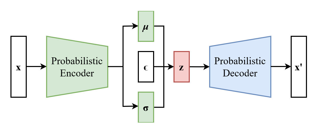
Now \(z\) is a deterministic function of \(\mu\), \(\sigma\) and an input \(\epsilon\) that carries no parameters. Gradients flow to \(\mu\) and \(\sigma\); the noise enters as data. The rest of the VAE was not new: the Helmholtz machine13 of 1995 already paired a recognition network (an encoder) with a generative one and a variational bound. What it lacked was a gradient of that bound with little noise, and this one line supplied it, in the VAE paper8 and, independently and at the same time, in Rezende, Mohamed and Wierstra12. The same trick appears throughout machine learning wherever a stochastic node sits inside a differentiable model.
Concretely, the gradient of the reconstruction term now reaches both encoder outputs through the chain rule:
The second one carries the tug of war: whatever the sign of \(\epsilon\), noise that made the reconstruction worse pushes \(\sigma\) down, while the KL term pushes it back toward 1. Step 3 of the lab runs this update, one sample at a time, and lands on the true posterior.
One VAE pass, number by number
Everything so far — the two heads, the trick, the two terms of the loss — in one network small enough to follow with a pencil: two inputs, a two-neuron encoder, a one-dimensional latent, a two-neuron decoder and two outputs. Step through the forward pass, then the backward one. The colours are the ones of the MLP chapter: green for the forward pass, orange for gradients, purple for weights. The second tab, Wider · 4-4-2-4-4, runs the same eleven steps on a network shaped like a real one: four inputs, four units on each side and a two-dimensional latent, where each dimension has its own \(\mu_k\), \(\sigma_k\) and \(\epsilon_k\) and every gradient is a matrix.
Three things to notice on the way:
- Steps 2, 3, 5 and 6 are an ordinary MLP. A VAE is two MLPs with a random number between them; every rule of backpropagation you already know applies unchanged.
- Step 4 is the only new operation, and step 10 is its derivative: \(\partial z/\partial \mu = 1\) and \(\partial z/\partial s = \tfrac12\sigma\epsilon\). Without the trick, step 10 would have nothing to multiply by and the encoder would get no gradient from the reconstruction at all.
- Step 10 is where the tug of war lives. Drag \(\epsilon\) and watch the reconstruction part of \(\partial L/\partial s\): it changes sign from draw to draw, but its average over \(\epsilon\), shown in the caption, is positive — noise costs reconstruction, so it pushes \(\sigma\) down. The KL part is the same for every \(\epsilon\) and always pushes \(\sigma\) towards 1.
Why the samples are blurry — and why it does not matter
Look back at chapter 16. The ELBO is a bound on the likelihood, so a VAE maximizes likelihood, so it optimizes forward KL, which is mode-covering. When the model cannot represent the data exactly it hedges — putting probability between the modes rather than choosing one.
Add the mechanical version: an \(\ell_2\) reconstruction loss is a Gaussian likelihood, and the optimal prediction under squared error is the conditional mean. If several sharp images are consistent with a code, the loss-minimizing output is their average. Averages of images are blurry. There is no bug here; the objective got exactly what it asked for.
So the blur is fixed by changing the objective, which is precisely what a production latent autoencoder does:
The perceptual term compares deep features rather than pixels, so a texture shifted by one pixel is not punished. The adversarial term — a GAN discriminator on the decoder output (chapter 18) — punishes exactly the smoothness that \(\ell_2\) rewards. Every latent autoencoder in every diffusion model is trained this way11.
What a VAE is actually for
Here is the deployment story, and it is not the one the textbook chapter implies.
A 512×512 RGB image is 786,432 numbers. Running diffusion there is unaffordable. Latent diffusion9 runs it in a compressed space instead — and a convolutional VAE is what compresses:
| Pixels | SD 1.5 / SDXL latent | SD 3 / FLUX latent | |
|---|---|---|---|
| Shape at 512×512 | \(512\times512\times3\) | \(64\times64\times4\) | \(64\times64\times16\) |
| Numbers | 786,432 | 16,384 | 65,536 |
| Compression | 1× | 48× | 12× |
The generative model never sees a pixel. It works entirely in the VAE's latent space, and the decoder turns the result back into an image at the very end. Three consequences worth carrying:
- The VAE caps your quality. Whatever the encoder cannot represent, the diffusion model cannot generate. Small text and fine texture are famously lost — and the move from 4 to 16 latent channels in SD3 and FLUX was aimed squarely at that.
- Its \(\beta\) is tiny. These are compressors: they are not sampled from directly, so the KL term only needs to keep the latent scale bounded and roughly regular. Practical values are around \(10^{-6}\).
- It is frozen. Train the autoencoder once, then keep it fixed while training the diffusion model. This is why a whole ecosystem of LoRAs and fine-tunes can share one latent space.
The other branch: discrete latents
Instead of a Gaussian latent, VQ-VAE10 snaps each latent vector to the nearest entry in a learned codebook. The latent becomes a grid of integers.
This is a different design with a different purpose, and the reason to know it is that it is what makes chapter 23 possible: once an image is a grid of integers, it is a sequence of tokens, and you can run a Transformer over it exactly as over text.
| KL-regularized (continuous) | VQ (discrete) | |
|---|---|---|
| Latent | Real-valued vectors | Codebook indices |
| Used by | Latent diffusion — SD, SDXL, SD3, FLUX | Autoregressive and masked generation — VQGAN, MaskGIT, Chameleon |
| Failure mode | Blur; limited capacity per channel | Codebook collapse — most entries never used |
| Why | Diffusion needs a continuous space to add noise to | Transformers need discrete tokens to predict |
Colab lab: the ELBO on a real VAE
The lab at the end of this page checks the ELBO on the worked example, where everything is exact. A Colab notebook takes the same questions to real VAEs on Fashion-MNIST (70 000 grayscale clothing images, 28 × 28). It runs in the browser, on CPU; there is nothing to install. Eight sections, each ending in a checkpoint with a check value:
- the evidence estimated by sampling, and why the ELBO is the log taken too early;
- the reparameterization gradient against autograd, and against the score function it replaced;
- the KL in closed form, from
torch.distributionsand by Monte Carlo; - a VAE on Fashion-MNIST, its two terms in nats, and the gradient at its two heads;
- β from 0 to 256: reconstruction, KL, active dimensions and how recognizable the prior samples are;
- posterior collapse at β = 1, caused by a decoder that does not need the code, and free bits;
- the gap on a real VAE: importance-weighted bounds and the amortization gap;
- your own configurations: does the best likelihood give the best samples?
Open the lab in Colab — save a copy to your Drive (File → Save a copy in Drive) to run and edit it.
Key takeaways
- An autoencoder compresses; it does not generate. Its latent space has holes, and you cannot see them.
- A VAE encodes a distribution per input and pulls those distributions toward a prior. That is what makes the space samplable.
- \(\log p(x) = \text{ELBO} + \text{KL}(q \,\|\, p(z \mid x))\). The ELBO is a lower bound on the evidence, the gap is how wrong the encoder is, and raising it trains encoder and decoder at once. Written out it is reconstruction minus KL-to-the-prior: both terms are necessary and they pull in opposite directions. It rewards the best trade, not the best reconstruction.
- β controls everything. Too small and it is an autoencoder; too large and the posterior collapses. Log the two terms separately.
- The reparameterization trick — \(z = \mu + \sigma\epsilon\) — is what makes the whole thing differentiable.
- Blur is the objective, not a bug: forward KL is mode-covering and \(\ell_2\) returns the conditional mean. Production autoencoders fix it with perceptual and adversarial losses.
- In 2026 a VAE is almost always the frozen compressor under a diffusion model, at 12 to 48× compression and a tiny β. It caps the quality of everything built on it.
- VQ-VAE is the discrete branch, and it is what makes autoregressive image generation possible.
Lab: the ELBO, measured
Four short experiments on the model of the worked example: \(p(z) = \mathcal{N}(0, 1)\), \(p(x \mid z) = \mathcal{N}(2z, 1)\), one observation \(x = 3\). It is small enough that the evidence \(\log p(x) = -2.6237\) and the posterior \(p(z \mid x) = \mathcal{N}(1.2,\ 0.2)\) are known exactly, which is never true in a real VAE — and that is the point. Every claim of this chapter becomes a number you can check. Everything runs with numpy alone: clone the scripts and change the constants.
Step 1 — the gap is the posterior error
Draw 10 000 random guesses \(q = \mathcal{N}(m, v)\) and compute, for each, the gap \(\log p(x) - \text{ELBO}\) and, separately, \(\text{KL}(q \,\|\, p(z \mid x))\) from the exact posterior.
q = N(m, v) | ELBO | log p(x) - ELBO | KL(q ‖ p(z∣x)) |
|---|---|---|---|
N(+1.87, 0.509) | -4.0504 | 1.4267 | 1.4267 |
N(+0.19, 0.481) | -5.4150 | 2.7914 | 2.7914 |
N(+2.29, 0.023) | -6.2543 | 3.6306 | 3.6306 |
N(+1.49, 0.008) | -3.9357 | 1.3120 | 1.3120 |
N(-1.53, 0.042) | -21.6319 | 19.0083 | 19.0083 |
N(1.20, 0.200) = p(z∣x) | -2.6237 | 0.0000 | 0.0000 |
10 000 random q | |
|---|---|
log p(x) | -2.6237 |
max ELBO found | -2.6240 |
q with ELBO > log p(x) | 0 |
max ∣gap - KL(q ‖ p(z∣x))∣ | 1.1e-14 |
"""Lab 1 — the gap between log p(x) and the ELBO is exactly KL(q || p(z|x)).

Toy model: p(z) = N(0, 1), p(x | z) = N(w z, s^2), w = 2, s = 1, x = 3.
Everything is Gaussian, so the evidence, the posterior and both KLs are exact.
The script draws 10 000 random q = N(m, v), computes the gap two ways, and
checks that no q ever beats log p(x).

Printed as a markdown table, in identifiers only, so one artifact serves both
the English and the Portuguese page.
"""

import numpy as np

W, S, X = 2.0, 1.0, 3.0
VAR_X = W**2 + S**2
LOG_PX = -0.5 * np.log(2 * np.pi * VAR_X) - X**2 / (2 * VAR_X)
M_POST, V_POST = W * X / VAR_X, S**2 / VAR_X      # p(z | x) = N(1.2, 0.2)


def elbo(m, v):
    rec = -0.5 * np.log(2 * np.pi * S**2) - ((X - W * m) ** 2 + W**2 * v) / (2 * S**2)
    kl = 0.5 * (m**2 + v - 1 - np.log(v))
    return rec - kl


def kl_gauss(m1, v1, m2, v2):
    """KL(N(m1, v1) || N(m2, v2))."""
    return 0.5 * (np.log(v2 / v1) + (v1 + (m1 - m2) ** 2) / v2 - 1)


rng = np.random.default_rng(42)
m = rng.uniform(-2, 3, 10_000)
v = np.exp(rng.uniform(-5, 1, 10_000))
gap = LOG_PX - elbo(m, v)
kl_post = kl_gauss(m, v, M_POST, V_POST)

print("| `q = N(m, v)` | `ELBO` | `log p(x) - ELBO` | `KL(q ‖ p(z∣x))` |")
print("|---|---:|---:|---:|")
for i in range(5):
    print(f"| `N({m[i]:+.2f}, {v[i]:.3f})` | {elbo(m[i], v[i]):.4f} | {gap[i]:.4f} | {kl_post[i]:.4f} |")
print(f"| `N({M_POST:.2f}, {V_POST:.3f})` = `p(z∣x)` | **{elbo(M_POST, V_POST):.4f}** | 0.0000 | 0.0000 |")
print()
print("| `10 000 random q` | |")
print("|---|---:|")
print(f"| `log p(x)` | {LOG_PX:.4f} |")
print(f"| `max ELBO found` | {elbo(m, v).max():.4f} |")
print(f"| `q with ELBO > log p(x)` | **{int((gap < 0).sum())}** |")
print(f"| `max ∣gap - KL(q ‖ p(z∣x))∣` | {np.abs(gap - kl_post).max():.1e} |")
The last two columns of the first table are the same number, and the largest disagreement over 10 000 guesses is \(10^{-14}\) — floating-point noise. That is step 2 of the derivation checked numerically: the gap is the KL to the posterior. No guess beats \(\log p(x)\), and the best of the 10 000 random ones stops 0.0003 short of it.
Try it
Set W = 0 in lab-1-gap.py: the decoder now ignores \(z\). What is the posterior, and what is the gap of \(q = p(z)\)? This is why posterior collapse is a stable state: once the decoder stops reading the code, returning the prior for every \(x\) is not a failure of the encoder — it is the correct answer.
Step 2 — one sample is enough
A VAE never computes \(\mathbb{E}_q[\log p(x \mid z)]\) exactly. It draws \(z = \mu + \sigma\epsilon\) and averages over \(K\) samples. How noisy is that, and how many samples does it need? The script repeats each estimate 2 000 times for the guess \(q_C = \mathcal{N}(1,\ 0.5^2)\), for the ELBO and for its gradient with respect to \(m\).
K (samples of z) | ELBO estimate: mean | std | dELBO/dm estimate: mean | std |
|---|---|---|---|---|
| 1 | -2.7955 | 1.2931 | 1.1103 | 2.0036 |
| 10 | -2.7312 | 0.3810 | 0.9792 | 0.6394 |
| 100 | -2.7396 | 0.1205 | 1.0021 | 0.2002 |
| 1000 | -2.7361 | 0.0375 | 0.9983 | 0.0607 |
exact | -2.7371 | 0 | 1.0000 | 0 |
"""Lab 2 — estimating the ELBO and its gradient with K samples of z.

Same toy model (p(z) = N(0,1), p(x|z) = N(2z, 1), x = 3), q = N(1, 0.5^2).
A VAE never computes E_q[log p(x|z)] exactly: it samples z = m + sigma * eps
and averages. Each estimate is repeated 2 000 times to measure its mean and
its spread. The KL term is kept in closed form, as in a real VAE.

Printed as a markdown table, in identifiers only, so one artifact serves both
the English and the Portuguese page.
"""

import numpy as np

W, S, X = 2.0, 1.0, 3.0
M, V = 1.0, 0.25
SIGMA = np.sqrt(V)
KL = 0.5 * (M**2 + V - 1 - np.log(V))
EXACT_REC = -0.5 * np.log(2 * np.pi * S**2) - ((X - W * M) ** 2 + W**2 * V) / (2 * S**2)
EXACT_ELBO = EXACT_REC - KL
EXACT_GRAD = W * (X - W * M) / S**2 - M          # d ELBO / d m


def log_lik(z):
    return -0.5 * np.log(2 * np.pi * S**2) - (X - W * z) ** 2 / (2 * S**2)


rng = np.random.default_rng(42)
REPEATS = 2_000

print("| `K` (samples of z) | `ELBO estimate: mean` | `std` | `dELBO/dm estimate: mean` | `std` |")
print("|---:|---:|---:|---:|---:|")
for k in (1, 10, 100, 1000):
    eps = rng.standard_normal((REPEATS, k))
    z = M + SIGMA * eps                               # the reparameterization trick
    elbo = log_lik(z).mean(1) - KL
    grad = (W * (X - W * z) / S**2).mean(1) - M       # dz/dm = 1, KL part = -m
    print(f"| {k} | {elbo.mean():.4f} | {elbo.std():.4f} | {grad.mean():.4f} | {grad.std():.4f} |")
print(f"| `exact` | **{EXACT_ELBO:.4f}** | 0 | **{EXACT_GRAD:.4f}** | 0 |")
The estimate is unbiased at every \(K\): the means sit on the exact values, \(-2.7371\) and \(1.0\), up to the noise of 2 000 repetitions. The spread falls like \(1/\sqrt{K}\) — 1.29, 0.38, 0.12, 0.04 — so a hundred times more samples buys ten times less noise. With \(K = 1\) a single gradient estimate can even have the wrong sign, and training still works: SGD only needs gradients that are right on average, and a minibatch of 128 images already averages 128 independent draws of \(\epsilon\). That is why every VAE uses one sample per image.
Try it
Set V = 0.01 (a narrow guess) and rerun. The spread at \(K = 1\) collapses. Why? Connect it to the \(4v\) in the reconstruction term: the noise of the estimator is the noise \(\sigma\epsilon\) the encoder chose to inject.
Step 3 — fitting q with the trick
Now train \(q\). Start at the prior (\(m = 0\), \(\log v = 0\)) and climb the ELBO by stochastic gradient ascent, one sample of \(\epsilon\) per step, with the two gradients of the reparameterization trick. The contours are the exact ELBO; the white line is what SGD sees.
"""Lab 3 — fitting q by stochastic gradient ascent, one sample of z per step.

Same toy model (p(z) = N(0,1), p(x|z) = N(2z, 1), x = 3). q = N(m, e^s)
starts at the prior (m = 0, s = 0) and climbs the ELBO with the
reparameterization trick and K = 1, exactly as a VAE encoder would, but for a
single x. The contours are the exact ELBO; the path is what SGD sees.
"""

from io import StringIO

import matplotlib.pyplot as plt
import numpy as np

W, S, X = 2.0, 1.0, 3.0
VAR_X = W**2 + S**2
M_POST, V_POST = W * X / VAR_X, S**2 / VAR_X


def elbo(m, s):
    v = np.exp(s)
    rec = -0.5 * np.log(2 * np.pi * S**2) - ((X - W * m) ** 2 + W**2 * v) / (2 * S**2)
    return rec - 0.5 * (m**2 + v - 1 - s)


rng = np.random.default_rng(42)
m, s, lr, steps = 0.0, 0.0, 0.02, 1500
path = [(m, s)]
for _ in range(steps):
    eps = rng.standard_normal()
    sigma = np.exp(s / 2)
    z = m + sigma * eps
    dz = W * (X - W * z) / S**2                        # d log p(x|z) / dz
    gm = dz * 1.0 - m                                  # reconstruction + KL parts
    gs = dz * 0.5 * sigma * eps - 0.5 * (np.exp(s) - 1)
    m, s = m + lr * gm, s + lr * gs                    # ascent: maximize the ELBO
    path.append((m, s))
path = np.array(path)
tail = path[-500:].mean(0)

mm, ss = np.meshgrid(np.linspace(-0.5, 2.5, 300), np.linspace(-6, 1, 300))
fig, ax = plt.subplots(figsize=(7.5, 4.6))
cs = ax.contourf(mm, ss, elbo(mm, ss), levels=np.linspace(-12, -2.6, 25), cmap="viridis", extend="min")
cs.set_rasterized(True)
fig.colorbar(cs, ax=ax, label="ELBO", ticks=[-12, -10, -8, -6, -4, -2.62])
ax.plot(path[:, 0], path[:, 1], c="w", lw=0.8, alpha=0.9)
ax.plot(*path[0], "o", c="C0", ms=9, mec="w", label="start: $p(z) = \\mathcal{N}(0, 1)$")
ax.plot(*tail, "o", mfc="none", mec="C3", mew=2.2, ms=17,
        label=f"SGD, mean of last 500 steps: $m = {tail[0]:.2f}$, $v = {np.exp(tail[1]):.2f}$")
ax.plot(M_POST, np.log(V_POST), "*", c="k", ms=14, mec="w", zorder=5,
        label=f"$p(z\\mid x) = \\mathcal{{N}}({M_POST:.1f},\\ {V_POST:.1f})$")
ax.plot(1.5, np.log(0.01), "s", c="C1", ms=8, mec="w", label="$q_B = \\mathcal{N}(1.5,\\ 0.1^2)$")
ax.set_xlabel("$m$ (mean of $q$)")
ax.set_ylabel("$s = \\log v$ (log-variance of $q$)")
ax.set_title(f"{steps} steps, $K = 1$, $\\eta = {lr}$")
ax.legend(loc="lower left", fontsize=8.5, framealpha=0.85)
fig.tight_layout()
buf = StringIO()
fig.savefig(buf, format="svg", transparent=True, dpi=110)
print(buf.getvalue())
The path heads straight up the slope and then wanders in a small cloud around the optimum, because each step sees only one \(\epsilon\). Averaged over its last 500 steps it sits at \(m = 1.20\), \(v = 0.20\): the true posterior, found without ever computing \(p(x)\) or \(p(z \mid x)\). The KL term alone would have kept it at the prior; the reconstruction alone would have driven it down to the square \(q_B\).
A real encoder does the same thing for every image at once, with one important difference: instead of free numbers \((m, s)\) per image it learns a function \(x \mapsto (\mu, \log\sigma^2)\) shared by all images. That function cannot land on every posterior exactly, and the leftover is called the amortization gap.
Try it
Change lr to 0.2 and then to 0.002. With the large step, look at the size of the cloud at the end; with the small one, check whether the path has arrived after 1 500 steps. That trade-off is the learning rate of a VAE.
Step 4 — β moves the optimum
Replace the ELBO by the \(\beta\)-weighted objective \(\mathbb{E}_q[\log p(x \mid z)] - \beta\,\text{KL}(q \,\|\, p(z))\). For this model the best guess has an exact formula, found by setting both derivatives to zero:
The first five columns are for \(x = 3\). The last averages the KL over a dataset of 10 000 observations \(x \sim p(x)\): it is how many nats about \(x\) the code keeps.
beta | m* | v* | E_q[log p(x∣z)] | KL(q ‖ p(z)) | mean KL over the dataset |
|---|---|---|---|---|---|
| 0.01 | 1.496 | 0.0025 | -0.924 | 3.618 | 3.121 |
| 0.1 | 1.463 | 0.0244 | -0.970 | 2.440 | 1.965 |
| 1 | 1.200 | 0.2000 | -1.499 | 1.125 | 0.805 |
| 4 | 0.750 | 0.5000 | -3.044 | 0.378 | 0.253 |
| 16 | 0.300 | 0.8000 | -5.399 | 0.057 | 0.037 |
| 100 | 0.058 | 0.9615 | -7.003 | 0.002 | 0.001 |
"""Lab 4 — what beta does to the best q, in closed form.

Same toy model (p(z) = N(0,1), p(x|z) = N(w z, s^2), w = 2, s = 1). Maximizing
E_q[log p(x|z)] - beta * KL(q || p(z)) over q = N(m, v) has an exact answer:

    m* = w x / (w^2 + beta s^2)        v* = beta s^2 / (w^2 + beta s^2)

The first block is the single observation x = 3. The second averages over a
whole dataset x ~ p(x): the mean KL(q || p(z)) is how many nats about x the
code keeps.

Printed as a markdown table, in identifiers only, so one artifact serves both
the English and the Portuguese page.
"""

import numpy as np

W, S, X = 2.0, 1.0, 3.0
BETAS = (0.01, 0.1, 1.0, 4.0, 16.0, 100.0)


def best_q(x, beta):
    m = W * x / (W**2 + beta * S**2)
    v = beta * S**2 / (W**2 + beta * S**2)
    return m, v


def terms(x, m, v):
    rec = -0.5 * np.log(2 * np.pi * S**2) - ((x - W * m) ** 2 + W**2 * v) / (2 * S**2)
    kl = 0.5 * (m**2 + v - 1 - np.log(v))
    return rec, kl


rng = np.random.default_rng(42)
data = W * rng.standard_normal(10_000) + S * rng.standard_normal(10_000)   # x ~ p(x)

print("| `beta` | `m*` | `v*` | `E_q[log p(x∣z)]` | `KL(q ‖ p(z))` | `mean KL over the dataset` |")
print("|---:|---:|---:|---:|---:|---:|")
for beta in BETAS:
    m, v = best_q(X, beta)
    rec, kl = terms(X, m, v)
    dm, dv = best_q(data, beta)
    mean_kl = terms(data, dm, dv)[1].mean()
    bold = "**" if beta == 1.0 else ""
    print(f"| {bold}{beta:g}{bold} | {m:.3f} | {v:.4f} | {rec:.3f} | {kl:.3f} | {mean_kl:.3f} |")
The three regimes of β is the whole story, as numbers:
- \(\beta \to 0\): \(v^* \to 0\) and \(m^* \to x/2 = 1.5\) — the point \(q_B\). Reconstruction is as good as it gets (\(-0.92\)) and the code keeps over 3 nats per observation. An autoencoder.
- \(\beta = 1\): \(\mathcal{N}(1.2,\ 0.2)\), the true posterior. The code keeps 0.805 nats on average — exactly \(\tfrac12\log 5\), the mutual information between \(x\) and \(z\) in this model.
- \(\beta \to \infty\): \(m^* \to 0\) and \(v^* \to 1\) — the prior. At \(\beta = 100\) the code keeps 0.001 nats: it says nothing about \(x\). Posterior collapse.
Here the decoder is fixed, so collapse is only the encoder giving up. In a real VAE the decoder learns too, and that makes it worse: once the codes carry nothing, the decoder learns to ignore them — and then, as the Try it of step 1 showed, the prior really is the best answer. That feedback loop is why collapse is hard to escape once it starts, and why KL annealing starts \(\beta\) at zero.
What the lab is actually teaching
The ELBO is not a loss someone guessed. It is \(\log p(x)\) minus a gap that you can measure, estimated with one noisy sample, climbed with the reparameterization trick, and bent by \(\beta\) toward either of two failures. Every VAE you train is this toy with more dimensions — the only difference is that you will never again see \(\log p(x)\) to check against.
Additional
Relation between Log Variance and Standard Deviation
Relation between Log Variance and Standard Deviation
- In VAEs, the encoder outputs the mean \( \mu \) and log variance \( \log(\sigma^2) \) of the latent space distribution.
- The standard deviation \( \sigma \) can be derived from the log variance using the relationship:
- The network predicts \(\log \sigma^2\) rather than \(\sigma\) because the log is unconstrained: an unbounded output maps to a guaranteed-positive variance, with no clipping and no risk of a negative standard deviation appearing halfway through training.
For \(z \sim \mathcal{N}(\mu, \sigma^2)\), write \(s = \log \sigma^2\) for the log-variance, as in the step-through diagram. Then
| Quantity | Symbol | In terms of \(s = \log \sigma^2\) |
|---|---|---|
| Variance | \(\sigma^2\) | \(e^{s}\) |
| Standard deviation | \(\sigma\) | \(e^{s/2}\) |
| Log-variance | \(s\) | \(2 \log \sigma\) |
The log scale is also numerically gentler: variances from \(10^{-4}\) to \(1\) are log-variances from \(-9.2\) to \(0\), a range a linear layer reaches without any extreme weight.
Appendix: the KL divergence
The Kullback–Leibler divergence4 shows up three times in this chapter — as the gap of the ELBO, as the term that pulls each code toward the prior, and in the forward-KL argument for blur — so it is worth knowing on its own.
What it measures
Read it as a procedure: draw \(x\) from \(q\), ask how much more probable \(q\) finds it than \(p\) does (on a log scale), and average. In information terms it is the number of extra nats per sample you pay when data that really comes from \(q\) is encoded with a code built for \(p\).
Three properties, all of them visible in the panel below:
- It is never negative, and it is zero only when \(q = p\) (Gibbs' inequality).
- It is not symmetric: in general \(\text{KL}(q \,\|\, p) \neq \text{KL}(p \,\|\, q)\), so it is not a distance.
- The integrand can be negative wherever \(p > q\), but the total never is.
Between two Gaussians
For two Gaussians the integral has a closed form:
Each piece has a meaning: the ratio of the two widths, the spread of \(q\) measured in units of \(p\), and the squared distance between the means, also in units of \(p\). Set \(p = \mathcal{N}(0, 1)\) and it becomes \(\tfrac12\big(\mu^2 + \sigma^2 - 1 - \log \sigma^2\big)\) — the KL term of the VAE loss, derived in step 5 from the expectation and here read off the general formula.
Move them yourself
Things to try:
- VAE posterior vs prior puts \(q = \mathcal{N}(1.2,\ 0.2)\), the exact posterior of the worked example, against the prior. \(\text{KL}(q \,\|\, p) = 1.1247\): the KL column of that example's table.
- Narrow q inside p gives \(\text{KL}(q \,\|\, p) = 0.318\) but \(\text{KL}(p \,\|\, q) = 0.807\). A narrow \(q\) sitting where \(p\) has mass is cheap in one direction and expensive in the other. That asymmetry is the mode-seeking versus mode-covering story of chapter 16.
- Far apart puts the means at \(\pm 2\) with equal widths: both directions give 8, because with equal spreads the KL is symmetric, \((\mu_q - \mu_p)^2 / 2\sigma^2\). Drag one of the widths and watch the two numbers split.
- Squeeze \(\sigma_q\) down to 0.25 on top of \(p = \mathcal{N}(0, 1)\): \(\text{KL}(q \,\|\, p)\) grows like \(\log(1/\sigma_q)\). That is the price a VAE pays for an encoder that turns into an autoencoder, one sharp point per input.
-
Sharma, A. “Introduction to Autoencoders,” PyImageSearch, 2023. ↩
-
Bandyopadhyay, H. "Autoencoders in Deep Learning: Tutorial & Use Cases," V7 Labs. ↩
-
Sharma, A. “A Deep Dive into Variational Autoencoders with PyTorch,” PyImageSearch, 2023. ↩
-
Higgins, I., et al. (2017). β-VAE: Learning Basic Visual Concepts with a Constrained Variational Framework — ICLR. Where the β knob is named and studied. ↩
-
Bowman, S., et al. (2016). Generating Sentences from a Continuous Space — CoNLL. The first careful account of posterior collapse, and of KL annealing as the fix. ↩
-
Variational AutoEncoders (VAE) with PyTorch — a clean, minimal implementation to read alongside this chapter. ↩
-
Kingma, D. P., & Welling, M. (2014). Auto-Encoding Variational Bayes — ICLR 2014 (on arXiv since December 2013). The ELBO and the reparameterization trick. ↩
-
Rombach, R., Blattmann, A., Lorenz, D., Esser, P., & Ommer, B. (2022). High-Resolution Image Synthesis with Latent Diffusion Models — CVPR. Stable Diffusion; section 3 is the autoencoder, and it is the part of the paper this chapter is about. ↩
-
van den Oord, A., Vinyals, O., & Kavukcuoglu, K. (2017). Neural Discrete Representation Learning — NeurIPS. VQ-VAE. ↩
-
Esser, P., Rombach, R., & Ommer, B. (2021). Taming Transformers for High-Resolution Image Synthesis — CVPR. VQGAN: the perceptual + adversarial recipe that made latent autoencoders sharp. ↩
-
Rezende, D. J., Mohamed, S., & Wierstra, D. (2014). Stochastic Backpropagation and Approximate Inference in Deep Generative Models — ICML. The same estimator, found independently. ↩
-
Dayan, P., Hinton, G. E., Neal, R. M., & Zemel, R. S. (1995). The Helmholtz Machine — Neural Computation 7(5). An encoder and a decoder trained against a variational bound, eighteen years before the VAE. ↩