7. Optimization
Gradient Descent is an optimization algorithm used to minimize the loss function in machine learning models. It works by iteratively adjusting the model parameters in the direction of the steepest descent of the loss function, as defined by the negative gradient.
The main idea behind gradient descent is to update the model parameters in the opposite direction of the gradient of the loss function with respect to the parameters. This is done using the following update rule:
Vanilla Gradient Descent
where:
- \(\theta\) represents the model parameters,
- \(\eta\) is the learning rate (a hyperparameter that controls the step size),
- \(\nabla J(\theta)\) is the gradient of the loss function with respect to the parameters.
In the standard Supervised Learning paradigm, the loss (per sample) is simply the output of the cost function. Machine Learning is mostly about optimizing functions (usually minimizing them). It could also involve finding Nash Equilibria between two functions like with GANs. This is done using Gradient Based Methods, though not necessarily Gradient Descent1.
A Gradient Based Method is a method/algorithm that finds the minima of a function, assuming that one can easily compute the gradient of that function. It assumes that the function is continuous and differentiable almost everywhere (it need not be differentiable everywhere)1.
Gradient Descent Intuition - Imagine being in a mountain in the middle of a foggy night. Since you want to go down to the village and have only limited vision, you look around your immediate vicinity to find the direction of steepest descent and take a step in that direction1.
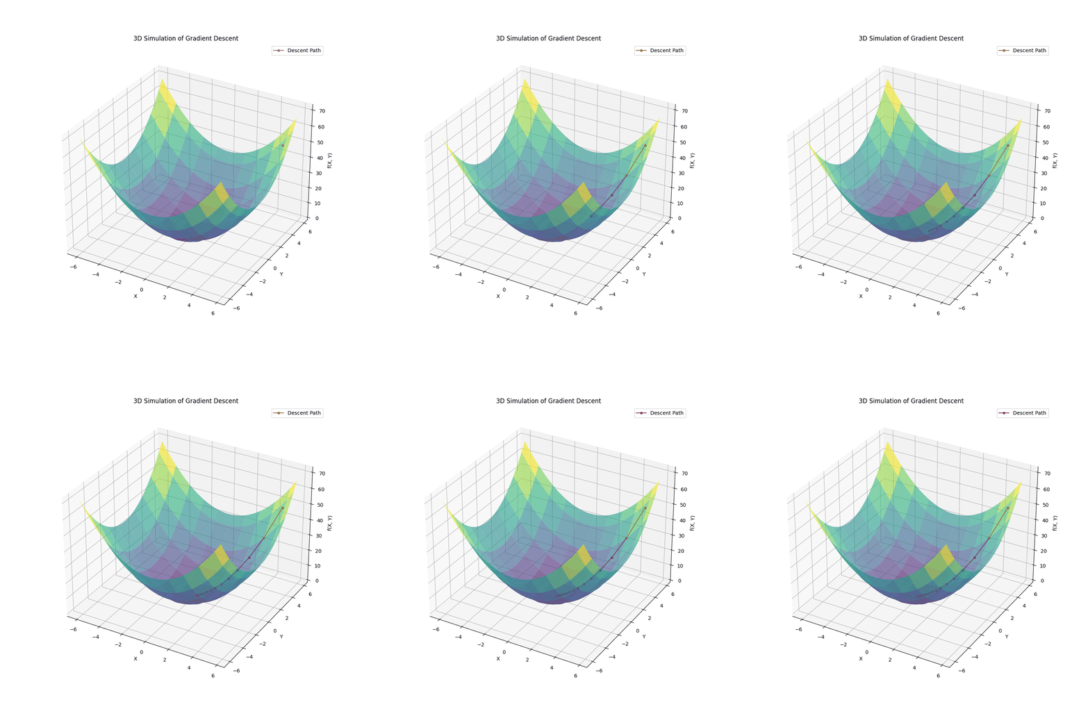
To visualize the gradient descent process, we can create a simple 3D plot that shows how the parameters of a model are updated over iterations to minimize a loss function. Below is an example code using Python with Matplotlib to create such a visualization.
Gradient Descent Variants
There are several variants of gradient descent, each with its own characteristics:
-
Batch Gradient Descent: Computes the gradient using the entire dataset. It provides a stable estimate of the gradient but can be slow for large datasets. Formula is given by:
\[ \theta = \theta - \eta \frac{1}{N} \sum_{i=1}^{N} \nabla J(\theta; x^{(i)}, y^{(i)}) \] -
Stochastic Gradient Descent (SGD): Computes the gradient using a single data point at a time. It introduces noise into the optimization process, which can help escape local minima but may lead to oscillations. Formula is given by:
\[ \theta_{t+1} = \theta_t - \eta \nabla J(\theta_t; x^{(i)}, y^{(i)}) \] -
Mini-Batch Gradient Descent: Combines the advantages of batch and stochastic gradient descent by using a small random subset of the data (mini-batch) to compute the gradient. It balances the stability of batch gradient descent with the speed of SGD.
\[ \theta_{t+1} = \theta_t - \eta \frac{1}{B} \sum_{i=1}^{B} \nabla J(\theta_t; x^{(i)}, y^{(i)}) \]
Momentum
Momentum is a variant of gradient descent that helps accelerate the optimization process by using the past gradients to smooth out the updates. It introduces a "momentum" term that accumulates the past gradients and adds it to the current gradient update. The update rule with momentum is given by:
In Momentum, we have two iterates (\(p\) and \(\theta\)) instead of just one. The updates are as follows:
\(V\) is called the SGD momentum. At each update step we add the stochastic gradient to the old value of the momentum, after dampening it by a factor \(\beta\) (value between 0 and 1). \(V\) can be thought of as a running average of the gradients. Finally we move \(\theta\) in the direction of the new momentum \(V\) 1.
Alternate Form: Stochastic Heavy Ball Method
This form is mathematically equivalent to the previous form. Here, the next step is a combination of previous step’s direction and the new negative gradient.
The momentum term helps to dampen oscillations and can lead to faster convergence, especially in scenarios with noisy gradients or ravines in the loss landscape.
RMSProp
RMSProp (Root Mean Square Propagation) is an adaptive learning rate optimization algorithm designed to address the diminishing learning rates of AdaGrad. It maintains a moving average of the squared gradients and uses this to normalize the gradients. The update rule is given by:
Where:
- \(V_t\) is the moving average of the squared gradients,
- \(\epsilon\) is a small constant added for numerical stability, helping to prevent division by zero.
ADAM Optimizer
ADAM (Adaptive Moment Estimation) is an advanced optimization algorithm that combines the benefits of both AdaGrad and RMSProp. It maintains two moving averages for each parameter: the first moment (mean) and the second moment (uncentered variance). The update rules are as follows:
- Compute the gradients:
- Update the first moment estimate:
- Update the second moment estimate:
- Compute bias-corrected estimates:
- Update the parameters:
Where:
- \(m_t\) is the first moment (the mean of the gradients),
- \(v_t\) is the second moment (the uncentered variance of the gradients),
- \(\beta_1\) and \(\beta_2\) are hyperparameters that control the decay rates of the moving averages,
- \(\epsilon\) is a small constant added for numerical stability. The default values for the hyperparameters are typically set to \(\beta_1 = 0.9\), \(\beta_2 = 0.999\), and \(\epsilon = 10^{-8}\)23.
ADAM is widely used in practice due to its adaptive learning rate properties and is particularly effective for training deep learning models.
Comparison
Here's a tabular comparison to highlight key differences:
| Gradient Descent (GD) | Stochastic Gradient Descent (SGD) | Momentum | ADAM | |
|---|---|---|---|---|
| Computational Cost per Update | High (full dataset) | Low (mini-batch) | Low (similar to SGD) | Medium (stores moments) |
| Convergence Speed | Slow (few updates) | Medium (many noisy updates) | Fast (accelerates in consistent directions) | Fast (adaptive + momentum) |
| Stability/Noise | High stability, low noise | Low stability, high noise | Medium stability, reduced oscillations | High stability, low effective noise |
| Adaptivity | None (fixed η) | None (fixed η, but can schedule) | Low (momentum helps indirectly) | High (per-parameter adaptation) |
| Best For | Small datasets, convex problems | Large datasets, online learning | Noisy gradients, ravine-like landscapes | Complex MLPs, sparse data |
| Common Hyperparameters | Learning rate (η) | Learning rate (η), batch size | Learning rate (η), momentum (β ~0.9) | Learning rate (η ~0.001), β1 (0.9), β2 (0.999), ε |
| Limitations | Scalability issues; stuck in local minima | Oscillations; requires tuning | Can overshoot; still fixed η | Potential overfitting; higher memory |
In summary,
- GD is basic but inefficient;
- SGD adds speed at the cost of noise;
- Momentum smooths SGD;
- and, ADAM offers the most automation and efficiency for MLPs, though SGD/Momentum may edge out in generalization for fine-tuned tasks.
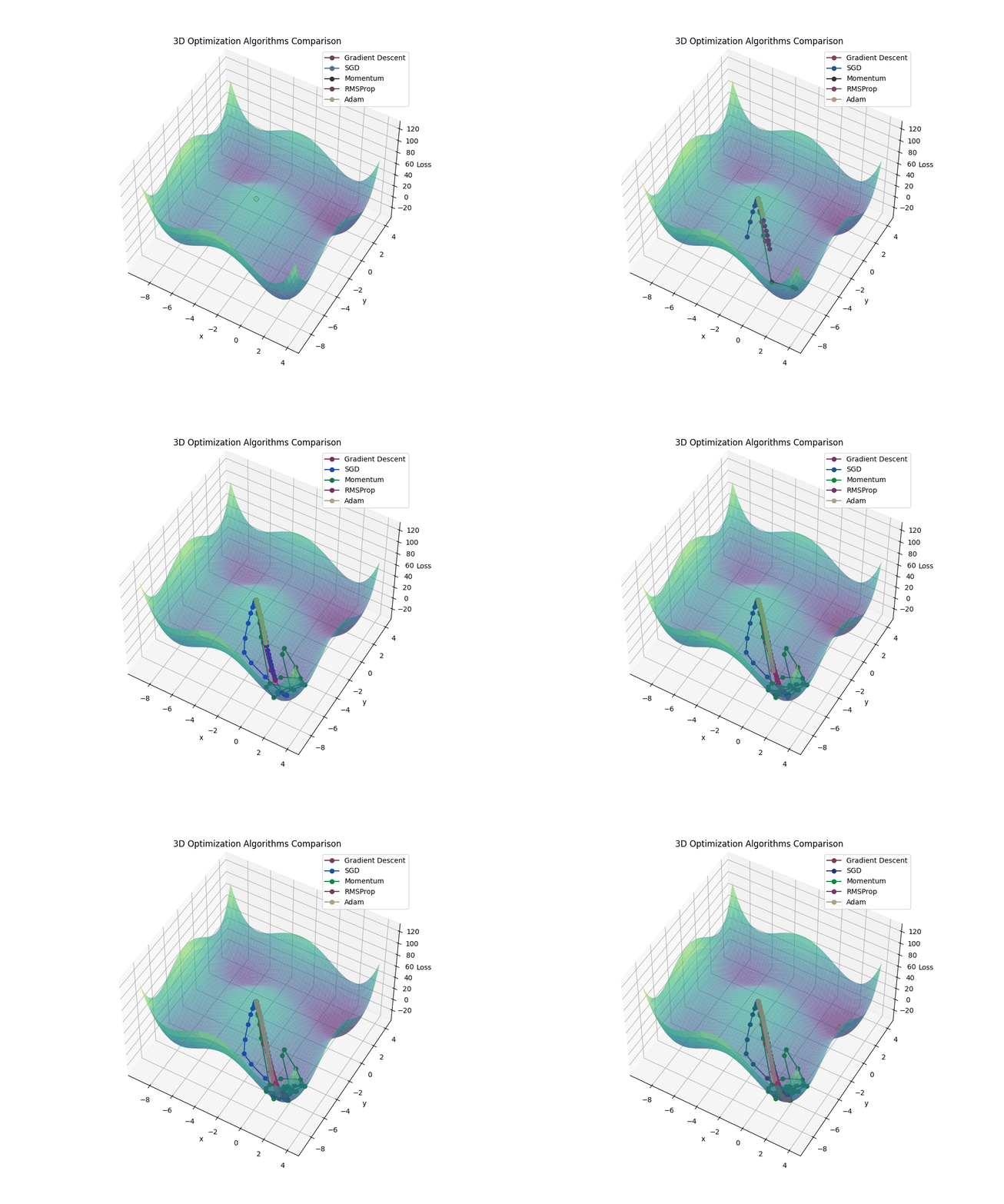
Choice depends on dataset size, computational resources, and problem complexity—experiment with validation sets for best results.
Additional Resources
-
Introduction to Gradient Descent and Backpropagation Algorithm, LeCun, Y. ↩↩↩↩
-
ADAM: A Method for Stochastic Optimization, Kingma, D. P., & Ba, J. ↩
-
Dive into Deep Learning, Zhang, A., & Lipton, Z. C. ↩