10. Deep Learning
O aprendizado profundo é um subconjunto do aprendizado de máquina que se concentra em treinar redes neurais artificiais com múltiplas camadas para aprender e fazer previsões a partir de dados complexos. Essas redes são inspiradas na estrutura do cérebro humano, onde "neurônios" processam informações e as passam adiante.
Diferentemente dos algoritmos de AM tradicionais, que frequentemente requerem engenharia manual de features, os modelos de aprendizado profundo extraem automaticamente features dos dados brutos por meio de camadas de processamento. Isso os torna poderosos para tarefas como reconhecimento de imagem, processamento de linguagem natural, síntese de fala e muito mais.
O aprendizado profundo se destaca com grandes conjuntos de dados e alto poder computacional (ex: GPUs), mas pode ser uma "caixa-preta" — às vezes é difícil interpretar por que um modelo toma uma decisão específica.
O bloco construtivo central é a rede neural artificial (ANN), que consiste em nós interconectados (neurônios) organizados em camadas. Os dados fluem da camada de entrada, através das camadas ocultas (onde está o "profundo"), até a camada de saída.
Componentes Principais
Uma rede neural típica tem três partes principais:
- Camada de Entrada: O ponto de entrada onde os dados brutos (ex: valores de pixels de uma imagem) são alimentados na rede. Não realiza cálculos; apenas passa os dados adiante.
- Camadas Ocultas: A "profundidade" do aprendizado profundo. São onde a mágica acontece — múltiplas camadas empilhadas que transformam os dados por meio de operações matemáticas. Cada camada aprende representações progressivamente mais abstratas.
- Camada de Saída: A camada final que produz a previsão ou classificação.
Diferentes Tipos de Camadas
Modelos de aprendizado profundo usam várias camadas especializadas dependendo da tarefa e arquitetura:
| Tipo de Camada | Descrição | Casos de Uso Comuns | Como Funciona |
|---|---|---|---|
| Densa (Totalmente Conectada) | Cada neurônio nesta camada é conectado a todos os neurônios da camada anterior. | Redes de propósito geral, como classificadores simples. | Aplica uma transformação linear (pesos × entradas + bias) seguida de uma função de ativação (ex: ReLU). |
| Convolucional | Usa filtros (kernels) para escanear dados de entrada, detectando padrões locais como bordas ou texturas. | Processamento de imagem e vídeo, visão computacional. | Desliza filtros sobre a entrada, calculando produtos internos para criar mapas de features. |
| Pooling | Reduz a amostra da saída das camadas convolucionais, reduzindo a carga computacional. | Após camadas convolucionais em CNNs. | Agrega valores em pequenas regiões (ex: grade 2×2) em um único valor. |
| Recorrente (ex: RNN, LSTM, GRU) | Lida com dados sequenciais mantendo uma "memória" de entradas anteriores via loops. | Previsão de séries temporais, PLN, reconhecimento de fala. | Processa entradas um passo por vez, usando estados ocultos para transportar informações. |
| Embedding | Converte dados categóricos (ex: palavras) em vetores densos de tamanho fixo. | PLN, sistemas de recomendação. | Mapeia dados esparsos de alta dimensionalidade para um espaço contínuo de menor dimensão. |
| Atenção | Permite ao modelo focar em partes relevantes da entrada dinamicamente. | PLN moderno (ex: modelos GPT), tradução automática. | Usa queries, keys e values para calcular pontuações de atenção. |
| Normalização | Estabiliza o treinamento normalizando as ativações dentro de uma camada. | Praticamente todas as redes profundas. | Ajusta e escala ativações (ex: média para 0, variância para 1). |
| Dropout | "Descarta" aleatoriamente uma fração de neurônios durante o treinamento para prevenir overfitting. | Regularização em qualquer rede. | Remove temporariamente conexões, forçando a rede a aprender representações redundantes. |
| Flatten | Converte dados multidimensionais em um vetor 1D para camadas densas. | Transição de extração de features (CNN) para classificação. | Reformata tensores sem alterar os valores. |
| Ativação | Aplica uma função não-linear à saída de outras camadas. | Em toda parte, para adicionar não-linearidade. | Transforma saídas lineares; ex: ReLU define valores negativos como 0. |
Arquiteturas Comuns de Aprendizado Profundo
Essas camadas são combinadas em arquiteturas adaptadas a problemas específicos:
- Redes Neurais Feedforward (FNN): Pilha básica de camadas densas para tarefas simples.
- Redes Neurais Convolucionais (CNN): Camadas convolucionais + pooling para dados espaciais como imagens (ex: ResNet, VGG).
- Redes Neurais Recorrentes (RNN): Camadas recorrentes para sequências (ex: LSTM para geração de texto).
- Transformers: Camadas de atenção para lidar com dependências de longo alcance (ex: BERT para PLN, Vision Transformers para imagens).
- Autoencoders: Encoder + decoder para aprendizado não supervisionado como denoising.
- GANs: Combina redes geradoras e discriminadoras para gerar dados realistas.
Passagem Direta e Reversa para Cada Camada
A passagem direta calcula a saída de cada camada dado o input, enquanto a passagem reversa calcula gradientes para aprendizado.
A retropropagação calcula o gradiente da perda em relação às entradas e parâmetros de cada camada para atualizá-los via otimizadores como o gradiente descendente.
A. Densa (Totalmente Conectada)
Every neuron in this layer is connected to every neuron in the previous layer. It's the most basic type. General-purpose networks, like simple classifiers or regressors. Often used in the final stages of more complex models.

A sample of a small fully-connected layer with four input and eight output neurons. Source: Linear/Fully-Connected Layers User's Guide
Parameters:
-
x: Input vector.
W: Weight matrix.
b: Bias vector.
-
\( x = [2, 3] \)
\( W = \begin{bmatrix} 1 & 2 \\ 0 & -1 \end{bmatrix} \)
\( b = [1, -1] \)
Forward Pass:
-
\( y = Wx + b \),
then apply activation (e.g., ReLU: \( y = \max(0, y) \)).
-
\( y = [9, -4] \),
ReLU: [9, 0].
Backward Pass:
-
-
Gradient w.r.t. input:
\( \displaystyle \frac{\partial L}{\partial x} = W^T \cdot \frac{\partial L}{\partial y'} \)
where \( y' \) is post-activation,
and \( \displaystyle \frac{\partial L}{\partial y'} \) is adjusted for activation,
e.g., for ReLU: 1 if \( y > 0 \), else 0).
-
Gradient w.r.t. weights:
\( \displaystyle \frac{\partial L}{\partial W} = \frac{\partial L}{\partial y'} \cdot x^T \).
-
Gradient w.r.t. bias:
\( \displaystyle \frac{\partial L}{\partial b} = \sum \frac{\partial L}{\partial y'} \).
-
-
Assume loss gradient \( \frac{\partial L}{\partial y'} = [0.5, -0.2] \) (post-ReLU). For ReLU: mask = [1, 0], so \( \frac{\partial L}{\partial y} = [0.5, 0] \).
-
\( \begin{align*} \displaystyle \frac{\partial L}{\partial x} &= W^T \cdot [0.5, 0] \\ & = \begin{bmatrix} 1 & 0 \\ 2 & -1 \end{bmatrix} \begin{bmatrix} 0.5 \\ 0 \end{bmatrix} \\ & = [0.5, 1.0] \end{align*} \).
-
\( \begin{align*} \displaystyle \frac{\partial L}{\partial W} &= [0.5, 0]^T \cdot [2, 3] \\ & = \begin{bmatrix} 1 & 1.5 \\ 0 & 0 \end{bmatrix} \end{align*} \).
-
\( \displaystyle \frac{\partial L}{\partial b} = [0.5, 0] \).
-
Implementation:
import numpy as np

def dense_forward(x, W, b):
    y_linear = np.dot(W, x) + b
    y = np.maximum(0, y_linear)  # ReLU
    return y, y_linear  # Cache linear for backprop

def dense_backward(dy_post_act, x, W, y_linear):
    # dy_post_act: ∂L/∂y (post-ReLU)
    dy_linear = dy_post_act * (y_linear > 0)  # ReLU derivative
    dx = np.dot(W.T, dy_linear)
    dW = np.outer(dy_linear, x)
    db = dy_linear
    return dx, dW, db

# Example
x = np.array([2, 3])
W = np.array([[1, 2], [0, -1]])
b = np.array([1, -1])
y, y_linear = dense_forward(x, W, b)
dy_post_act = np.array([0.5, -0.2])
dx, dW, db = dense_backward(dy_post_act, x, W, y_linear)
print("Forward y:", y)  # [9, 0]
print("dx:", dx)  # [0.5, 1.0]
print("dW:", dW)  # [[1, 1.5], [0, 0]]
print("db:", db) # [0.5, 0]B. Convolucional
Uses filters (kernels) to scan input data, detecting local patterns like edges or textures. Key to "convolutional neural networks" (CNNs). Image and video processing, computer vision (e.g., object detection in photos). Slides filters over the input, computing dot products to create feature maps. Reduces spatial dimensions while preserving important features.

Convolution of an image with an edge detector convolution kernel. Sources: Deep Learning in a Nutshell: Core Concepts
Calculating convolution by sliding image patches over the entire image. One image patch (yellow) of the original image (green) is multiplied by the kernel (red numbers in the yellow patch), and its sum is written to one feature map pixel (red cell in convolved feature). Image source: Deep Learning in a Nutshell: Core Concepts
Parameters:
-
X: Input matrix (e.g., image).
K: Convolution kernel (filter).
b: Bias term.
-
(2D, stride=1, no padding):
\( X = \begin{bmatrix} 1 & 2 & 3 \\ 4 & 5 & 6 \\ 7 & 8 & 9 \end{bmatrix} \)
\( K = \begin{bmatrix} 1 & 0 \\ -1 & 1 \end{bmatrix} \)
\( b=1 \)
Forward Pass:
-
Convolution:
\( \displaystyle Y[i,j] = \sum_{m,n} X[i+m, j+n] \cdot K[m,n] + b \).
-
Convolution:
\( \begin{bmatrix} \begin{array}{ll} =& 1 \times 1 + 2 \times 0 \\ &+ 4 \times (-1) + 5 \times 1 \\ &+ 1 \end{array} & \begin{array}{ll} =& 2 \times 1 + 3 \times 0 \\ &+ 5 \times (-1) + 6 \times 1 \\ &+ 1 \end{array} \\ \begin{array}{ll} =& 4 \times 1 + 5 \times 0 \\ &+ 7 \times (-1) + 8 \times 1 \\ &+ 1 \end{array} & \begin{array}{ll} =& 5 \times 1 + 6 \times 0 \\ &+ 8 \times (-1) + 9 \times 1 \\ &+ 1 \end{array} \end{bmatrix} \)
\( Y = \begin{bmatrix} 3 & 3 \\ -1 & -1 \end{bmatrix} \)
Backward Pass:
-
-
Gradient w.r.t. input:
Convolve upstream gradient \( \displaystyle \frac{\partial L}{\partial Y} \) with rotated kernel (full convolution).
-
Gradient w.r.t. kernel:
Convolve input \( X \) with \( \displaystyle \frac{\partial L}{\partial Y} \).
-
Gradient w.r.t. bias:
Sum of \( \displaystyle \frac{\partial L}{\partial Y} \).
-
-
\( \displaystyle \frac{\partial L}{\partial Y} = \begin{bmatrix} 0.5 & -0.5 \\ 1 & 0 \end{bmatrix} \).
-
\( \displaystyle \frac{\partial L}{\partial X} \):
Full conv with rotated K (\( \begin{bmatrix} 1 & -1 \\ 0 & 1 \end{bmatrix} \)) and padded \( dY \), approx. \( \begin{bmatrix} 0.5 & -0.5 & -0.5 \\ 0 & 1.5 & 0 \\ 1 & 0 & 0 \end{bmatrix} \) (simplified calc).
-
\( \displaystyle \frac{\partial L}{\partial K} = \) Conv X with dY:
\( \begin{bmatrix} 0.5*1 + (-0.5)*2 + 1*4 + 0*5 \\ \ldots \end{bmatrix} \)
(detailed in code).
-
\( \displaystyle \frac{\partial L}{\partial b} = 0.5 -0.5 +1 +0 = 1 \).
-
Implementation:
import numpy as np
from scipy.signal import correlate2d, convolve2d

def conv_forward(X, K, b):
    Y = correlate2d(X, K, mode='valid') + b  # SciPy correlate for conv
    return Y, X  # Cache X

def conv_backward(dY, X, K):
    # Rotate kernel 180 degrees for full conv
    K_rot = np.rot90(K, 2)
    # Pad dY to match X shape for dx
    pad_h, pad_w = K.shape[0]-1, K.shape[1]-1
    dY_padded = np.pad(dY, ((pad_h//2, pad_h-pad_h//2), (pad_w//2, pad_w-pad_w//2)))
    dX = convolve2d(dY_padded, K_rot, mode='valid')
    dK = correlate2d(X, dY, mode='valid')
    db = np.sum(dY)
    return dX, dK, db

# Example
X = np.array([[1,2,3],[4,5,6],[7,8,9]])
K = np.array([[1,0],[-1,1]])
b = 1
Y, _ = conv_forward(X, K, b)
dY = np.array([[0.5, -0.5],[1, 0]])
dX, dK, db = conv_backward(dY, X, K)
print("Forward Y:\n", Y)
print("dX:\n", dX)
print("dK:\n", dK)
print("db:", db)C. Pooling (Max Pooling)
Reduz a amostra da saída das camadas convolucionais, reduzindo a carga computacional e prevenindo overfitting. Segue as camadas convolucionais em CNNs para resumir features. Agrega valores em pequenas regiões (ex: grade 2×2) em um único valor, tornando o modelo mais robusto a variações como translações.
Passagem Direta:
-
\(Y[i,j] = \max(X[i:i+k, j:j+k])\) para tamanho de pool \(k\).
-
\(X = \begin{bmatrix} 1 & 2 & 3 & 4 \\ 5 & 6 & 7 & 8 \\ 9 & 10 & 11 & 12 \\ 13 & 14 & 15 & 16 \end{bmatrix}\), pool=2, stride=2,
\(Y = \begin{bmatrix} 6 & 8 \\ 14 & 16 \end{bmatrix}\).
Passagem Reversa:
-
Distribua o gradiente upstream \(\frac{\partial L}{\partial Y}\) para a posição máxima em cada janela; 0 nos demais.
-
\(\frac{\partial L}{\partial Y} = \begin{bmatrix} 0.5 & -0.5 \\ 1 & 0 \end{bmatrix}\): 0,5 para a posição de 6 (1,1), -0,5 para 8 (1,3), etc.
Implementação:
import numpy as np

def max_pool_forward(X, pool_size=2, stride=2):
    H, W = X.shape
    out_H, out_W = H // stride, W // stride
    Y = np.zeros((out_H, out_W))
    max_idx = np.zeros_like(X, dtype=bool)  # For backprop
    for i in range(0, H, stride):
        for j in range(0, W, stride):
            slice = X[i:i+pool_size, j:j+pool_size]
            max_val = np.max(slice)
            Y[i//stride, j//stride] = max_val
            max_idx[i:i+pool_size, j:j+pool_size] = (slice == max_val)
    return Y, max_idx

def max_pool_backward(dY, max_idx, pool_size=2, stride=2):
    dX = np.zeros_like(max_idx, dtype=float)
    for i in range(dY.shape[0]):
        for j in range(dY.shape[1]):
            dX[i*stride:i*stride+pool_size, j*stride:j*stride+pool_size] = dY[i,j] * max_idx[i*stride:i*stride+pool_size, j*stride:j*stride+pool_size]
    return dX

# Example
X = np.arange(1,17).reshape(4,4)
Y, max_idx = max_pool_forward(X)
dY = np.array([[0.5, -0.5],[1, 0]])
dX = max_pool_backward(dY, max_idx)
print("Forward Y:\n", Y)
print("dX:\n", dX)D. Recorrente (LSTM)
Recurrent Neural Networks (RNNs) are powerful for sequence data. Long Short-Term Memory (LSTM) networks are a type of RNN designed to capture long-term dependencies and mitigate issues like vanishing gradients.
Parameters:
-
(Simplified to hidden size=1 for clarity):
-
Inputs:
\( x_t = [0.5] \),
\( h_{t-1} = [0.1] \),
\( C_{t-1} = [0.2] \)
-
Weights:
\( W_f = [[0.5, 0.5]] \),
\( W_i = [[0.4, 0.4]] \),
\( W_C = [[0.3, 0.3]] \),
\( W_o = [[0.2, 0.2]] \)
-
Biases: \( b_f = b_i = b_C = b_o = [0.0] \)
-
Forward Pass:
-
- Concatenate: \( \text{concat} = [h_{t-1}, x_t] \)
- Forget gate: \( f_t = \sigma(W_f \cdot \text{concat} + b_f) \)
- Input gate: \( i_t = \sigma(W_i \cdot \text{concat} + b_i) \)
- Cell candidate: \( \tilde{C}_t = \tanh(W_C \cdot \text{concat} + b_C) \)
- Cell state: \( C_t = f_t \cdot C_{t-1} + i_t \cdot \tilde{C}_t \)
- Output gate: \( o_t = \sigma(W_o \cdot \text{concat} + b_o) \)
- Hidden state: \( h_t = o_t \cdot \tanh(C_t) \)
-
- concat = [0.1, 0.5]
- \( f_t = \sigma(0.3) \approx 0.5744 \)
- \( i_t = \sigma(0.24) \approx 0.5597 \)
- \( \tilde{C}_t = \tanh(0.18) \approx 0.1785 \)
- \( C_t \approx 0.5744 \cdot 0.2 + 0.5597 \cdot 0.1785 \approx 0.2146 \)
- \( o_t = \sigma(0.12) \approx 0.5300 \)
- \( h_t \approx 0.5300 \cdot \tanh(0.2146) \approx 0.1120 \)
Backward Pass:
-
Gradients are computed via chain rule:
- \( dC_t = dh_t \cdot o_t \cdot (1 - \tanh^2(C_t)) + dC_{next} \) (dC_next from future timestep)
- \( do_t = dh_t \cdot \tanh(C_t) \cdot \sigma'(o_t) \)
- \( d\tilde{C}_t = dC_t \cdot i_t \cdot (1 - \tilde{C}_t^2) \)
- \( di_t = dC_t \cdot \tilde{C}_t \cdot \sigma'(i_t) \)
- \( df_t = dC_t \cdot C_{t-1} \cdot \sigma'(f_t) \)
- \( dC_{prev} = dC_t \cdot f_t \)
- Then, backpropagate to concat: \( d\text{concat} = W_o^T \cdot do_t + W_C^T \cdot d\tilde{C}_t + W_i^T \cdot di_t + W_f^T \cdot df_t \)
- Split \( d\text{concat} \) into \( dh_{prev} \) and \( dx_t \)
- Parameter gradients: \( dW_f = df_t \cdot \text{concat}^T \), \( db_f = df_t \), and similarly for others.
-
(Assume upstream: \( dh_t = [0.1] \), \( dC_t = [0.05] \) from next timestep):
- \( dC_t \approx 0.1 \cdot 0.5300 \cdot (1 - \tanh^2(0.2146)) + 0.05 \approx 0.1028 + 0.05 = 0.1528 \) (detailed steps in code output)
- Resulting gradients match the executed values below (e.g., \( dx_t \approx [0.0216] \), etc.).
import numpy as np

def sigmoid(x):
    return 1 / (1 + np.exp(-x))

def dsigmoid(y):
    return y * (1 - y)

def tanh(x):
    return np.tanh(x)

def dtanh(y):
    return 1 - y**2

# Forward pass
def lstm_forward(x_t, h_prev, C_prev, W_f, W_i, W_C, W_o, b_f, b_i, b_C, b_o):
    concat = np.concatenate((h_prev, x_t), axis=0)
    f_t = sigmoid(np.dot(W_f, concat) + b_f)
    i_t = sigmoid(np.dot(W_i, concat) + b_i)
    C_tilde = tanh(np.dot(W_C, concat) + b_C)
    C_t = f_t * C_prev + i_t * C_tilde
    o_t = sigmoid(np.dot(W_o, concat) + b_o)
    h_t = o_t * tanh(C_t)
    cache = (concat, f_t, i_t, C_tilde, o_t, C_t)
    return h_t, C_t, cache

# Backward pass
def lstm_backward(dh_next, dC_next, cache, W_f, W_i, W_C, W_o):
    concat, f_t, i_t, C_tilde, o_t, C_t = cache

    # Derivatives
    dC_t = dh_next * o_t * dtanh(tanh(C_t)) + dC_next
    do_t = dh_next * tanh(C_t) * dsigmoid(o_t)
    dC_tilde = dC_t * i_t * dtanh(C_tilde)
    di_t = dC_t * C_tilde * dsigmoid(i_t)
    df_t = dC_t * C_prev * dsigmoid(f_t)
    dC_prev = dC_t * f_t

    # Gradients for gates
    dconcat_o = np.dot(W_o.T, do_t)
    dconcat_C = np.dot(W_C.T, dC_tilde)
    dconcat_i = np.dot(W_i.T, di_t)
    dconcat_f = np.dot(W_f.T, df_t)
    dconcat = dconcat_f + dconcat_i + dconcat_C + dconcat_o

    # Split for h_prev and x_t
    hidden_size = h_prev.shape[0]
    dh_prev = dconcat[:hidden_size]
    dx_t = dconcat[hidden_size:]

    # Parameter gradients
    dW_f = np.outer(df_t, concat)
    db_f = df_t
    dW_i = np.outer(di_t, concat)
    db_i = di_t
    dW_C = np.outer(dC_tilde, concat)
    db_C = dC_tilde
    dW_o = np.outer(do_t, concat)
    db_o = do_t

    return dx_t, dh_prev, dC_prev, dW_f, db_f, dW_i, db_i, dW_C, db_C, dW_o, db_o

# Numerical example (hidden size = 1)
x_t = np.array([0.5])
h_prev = np.array([0.1])
C_prev = np.array([0.2])
W_f = np.array([[0.5, 0.5]])
W_i = np.array([[0.4, 0.4]])
W_C = np.array([[0.3, 0.3]])
W_o = np.array([[0.2, 0.2]])
b_f = np.array([0.0])
b_i = np.array([0.0])
b_C = np.array([0.0])
b_o = np.array([0.0])

# Forward
h_t, C_t, cache = lstm_forward(x_t, h_prev, C_prev, W_f, W_i, W_C, W_o, b_f, b_i, b_C, b_o)
print("Forward h_t:", h_t)  # Output: [0.11199714]
print("Forward C_t:", C_t)  # Output: [0.2145628]

# Backward example: assume dh_next = [0.1], dC_next = [0.05]
dh_next = np.array([0.1])
dC_next = np.array([0.05])
dx_t, dh_prev, dC_prev, dW_f, db_f, dW_i, db_i, dW_C, db_C, dW_o, db_o = lstm_backward(dh_next, dC_next, cache, W_f, W_i, W_C, W_o)

print("Backward dx_t:", dx_t)  # Output: [0.02164056]
print("Backward dh_prev:", dh_prev)  # Output: [0.02164056]
print("Backward dC_prev:", dC_prev)  # Output: [0.05780591]
print("Backward dW_f:", dW_f)  # Output: [[0.00049199 0.00245997]]
print("Backward db_f:", db_f)  # Output: [0.00491995]
print("Backward dW_i:", dW_i)  # Output: [[0.00044162 0.00220808]]
print("Backward db_i:", db_i)  # Output: [0.00441615]
print("Backward dW_C:", dW_C)  # Output: [[0.00545376 0.02726878]]
print("Backward db_C:", db_C)  # Output: [0.05453756]
print("Backward dW_o:", dW_o)  # Output: [[0.00052643 0.00263213]]
print("Backward db_o:", db_o) # Output: [0.00526427]Notes
- This is a single-timestep LSTM with hidden size 1 for simplicity. In practice, LSTMs process sequences (multiple timesteps) and have larger hidden sizes; backpropagation through time (BPTT) unrolls the network over timesteps.
- The code uses NumPy; for real models, use PyTorch or TensorFlow for automatic differentiation and batching.
- Outputs are approximate due to floating-point precision but match the manual calculations.
- If you need a multi-timestep example, sequence processing, or integration into a full RNN, let me know!
E. Embedding
Passagem Direta: \(y = E[i]\), onde \(E\) é a matriz de embedding e \(i\) é o índice de entrada.
Passagem Reversa: Gradiente \(\frac{\partial L}{\partial E[i]} += \frac{\partial L}{\partial y}\); outras linhas 0. (Atualização esparsa).
Implementação:
import numpy as np

def embedding_forward(index, E):
    return E[index]

def embedding_backward(dy, index, E_shape):
    dE = np.zeros(E_shape)
    dE[index] = dy
    return dE

# Example
E = np.array([[0.1,0.2,0.3],[0.4,0.5,0.6]])
index = 1
y = embedding_forward(index, E)
dy = np.array([0.1, -0.1, 0.2])
dE = embedding_backward(dy, index, E.shape)
print("dE:\n", dE)
F. Atenção (Produto Escalar Escalado)
Passagem Direta: \(\text{Attention} = \text{softmax}\left(\frac{QK^T}{\sqrt{d}}\right)V\).
Passagem Reversa: Gradientes para Q, K, V via regra da cadeia no softmax e multiplicações de matrizes.
Implementação:
import numpy as np

def softmax(x):
    exp_x = np.exp(x - np.max(x, axis=-1, keepdims=True))
    return exp_x / np.sum(exp_x, axis=-1, keepdims=True)

def attention_forward(Q, K, V):
    d = Q.shape[-1]
    scores = np.dot(Q, K.T) / np.sqrt(d)
    weights = softmax(scores)
    attn = np.dot(weights, V)
    return attn, (scores, weights, K, V)  # Cache

def attention_backward(dattn, cache):
    scores, weights, K, V = cache
    dweights = np.dot(dattn, V.T)
    dscores = weights * (dweights - np.sum(weights * dweights, axis=-1, keepdims=True))
    dQ = np.dot(dscores, K) / np.sqrt(K.shape[-1])
    dK = np.dot(dscores.T, Q) / np.sqrt(K.shape[-1])
    dV = np.dot(weights.T, dattn)
    return dQ, dK, dV

# Example
Q = K = V = np.array([[1.,0.],[0.,1.]])
attn, cache = attention_forward(Q, K, V)
dattn = np.array([[0.1,0.2],[ -0.1,0.3]])
dQ, dK, dV = attention_backward(dattn, cache)
print("dQ:\n", dQ)G. Normalização (Batch Normalization)
Passagem Direta: Normalizar, escalar, deslocar.
Passagem Reversa: Gradientes para entrada, gamma, beta via regra da cadeia sobre média/variância.
Implementação:
import numpy as np

def batch_norm_forward(x, gamma, beta, epsilon=1e-4):
    mu = np.mean(x)
    var = np.var(x)
    x_hat = (x - mu) / np.sqrt(var + epsilon)
    y = gamma * x_hat + beta
    return y, (x_hat, mu, var)

def batch_norm_backward(dy, cache, gamma):
    x_hat, mu, var = cache
    N = dy.shape[0]
    dx_hat = dy * gamma
    dvar = np.sum(dx_hat * (x - mu) * -0.5 * (var + epsilon)**(-1.5), axis=0)
    dmu = np.sum(dx_hat * -1 / np.sqrt(var + epsilon), axis=0) + dvar * np.mean(-2 * (x - mu), axis=0)
    dx = dx_hat / np.sqrt(var + epsilon) + dvar * 2 * (x - mu) / N + dmu / N
    dgamma = np.sum(dy * x_hat, axis=0)
    dbeta = np.sum(dy, axis=0)
    return dx, dgamma, dbeta

# Example
x = np.array([1,2,3,4.])
gamma, beta = 1, 0
y, cache = batch_norm_forward(x, gamma, beta)
dy = np.array([0.1,0.2,-0.1,0.3])
dx, dgamma, dbeta = batch_norm_backward(dy, cache, gamma)
print("dx:", dx)
print("dgamma:", dgamma)
print("dbeta:", dbeta)H. Dropout
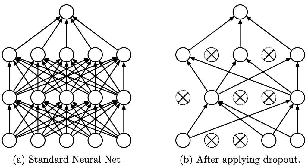
Dropout Neural Net Model. Left: A standard neural net with 2 hidden layers. Right: An example of a thinned net produced by applying dropout to the network on the left. Crossed units have been dropped. Source: Dropout: A Simple Way to Prevent Neural Networks from Overfitting
Forward Pass: Mask during training.
Backward Pass: Same mask applied to upstream gradient (scale by 1/(1-p)).
Numerical Example: Same as forward; backward passes dy through mask.
Implementation:
import numpy as np

def dropout_forward(x, p, training=True):
    if training:
        mask = np.random.binomial(1, 1-p, size=x.shape) / (1-p)
        y = x * mask
        return y, mask
    return x, None

def dropout_backward(dy, mask):
    if mask is None:
        return dy
    return dy * mask

# Example
np.random.seed(0)
x = np.array([1,2,3,4.])
p = 0.5
y, mask = dropout_forward(x, p)
dy = np.array([0.1,0.2,0.3,0.4])
dx = dropout_backward(dy, mask)
print("dx:", dx)I. Flatten
Passagem Direta: Reformatar para 1D.
Passagem Reversa: Reformatar o gradiente upstream de volta ao formato original.
Implementação:
import numpy as np

def flatten_forward(x):
    return x.flatten(), x.shape

def flatten_backward(dy, orig_shape):
    return dy.reshape(orig_shape)

# Example
x = np.array([[1,2],[3,4]])
y, shape = flatten_forward(x)
dy = np.array([0.1,0.2,0.3,0.4])
dx = flatten_backward(dy, shape)
print("dx:\n", dx)
J. Ativação (ReLU)
Passagem Direta: \(y = \max(0, x)\).
Passagem Reversa: \(\frac{\partial L}{\partial x} = \frac{\partial L}{\partial y} \cdot (x > 0)\).
Implementação:
import numpy as np

def relu_forward(x):
    return np.maximum(0, x), x

def relu_backward(dy, x_cache):
    return dy * (x_cache > 0)

# Example
x = np.array([-1,0,2,-3])
y, x_cache = relu_forward(x)
dy = np.array([0.5,-0.5,1,0])
dx = relu_backward(dy, x_cache)
print("dx:", dx)
-
Mohd Halim Mohd Noor, Ayokunle Olalekan Ige: A Survey on State-of-the-art Deep Learning Applications and Challenges, 2025. ↩
-
Aston Zhang et al.: Dive into Deep Learning, 2020. ↩
-
Ian Goodfellow, Yoshua Bengio, Aaron Courville: Deep Learning, 2016. ↩